Parametric density estimation, a.k.a fitting probability distribution to observed data by tweaking the parameters of the distribution’s functional form, is all the rage now with generative modeling and LLMs. I think nonparametric methods deserve some love too and I hope to give a very small primer on these methods in a series of posts.
What are Nonparametric methods?
Looking at the name, you might have guessed that these are methods where you fit a probability distribution to data without any underlying parameters that are computed from the data itself.
Why bother? This is a very good question in the current age of deep learning where we have parametric function approximators (the neural networks) that can approximate any reasonable function (including a probability distribution.) However, in the regime of small data, where these large networks can easily overfit, these nonparametric methods are very useful. Furthermore, I often use them to quickly get an initial sense of my data – how many modes does the underlying distribution have, where does the mean lie, what sort of variance does the data exhibit, etc. In light of these advantages, I claim that it is useful to understand nonparametric methods and how to implement them.
Density Estimation
I learned this neat intuition from Chris Bishop’s textbook. Suppose we are trying to estimate a probability density $p(x)$ where $x \in \mathbb{R}^D$. Given a region $R$, we can compute the probability mass associated with this region as
$$ P = \int_{R} p(x) dx $$
Given a dataset of $N$ points drawn from $p(x)$, the average number of points $K$ that lie within region $R$ is
$$ K = NP $$
Now comes the crucial argument: If the region $R$ is small enough that we can assume the density $p(x)$ is roughly constant over the region, then we have
$$ P = p(x)V $$
where $V$ is the volume of the region R. Combining the above two equations, we get
$$ p(x) = \frac{K}{NV} $$
The above result gives us two strategies to estimate $p(x)$ for any point $x \in \mathbb{R}^D$:
- We can fix $V$ and determine $K$ from data
- We can fix $K$ and determine $V$ from data
All nonparametric density estimation methods can be viewed through the lens of the above two strategies. We describe Histograms, a nonparametric method, below.
Histograms
Following strategy 1 above, let’s discretize each of the $D$ dimensions of $\mathbb{R}^D$ into bins of width $\Delta$. Note that each bin has a fixed volume $V = \Delta^D$. To compute the density $p(x)$, all we need to do is to determine $K$ from data.
Let me demonstrate how histograms work with a 1-D example
import matplotlib.pyplot as plt
import numpy as np
from scipy.stats import norm
plt.rcParams["figure.figsize"] = (5,2)

# Mixture of 2 Gaussians
pdf = lambda x: 0.7 * norm.pdf(x, 0.5, 0.1) + 0.3 * norm.pdf(x, 1, 0.1)

dx = 1e-2
xaxis = np.arange(0.25, 1.25, dx)
plt.plot(xaxis, list(map(pdf, xaxis)), label="p(x)")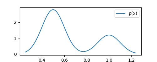
The above plot shows the density $p(x)$ that we want to estimate. Remember, we do not know this distribution. However, we do have $N$ observations drawn from it. Let’s plot these observations
N = 100
np.random.seed(0)
def sample():
    if np.random.rand() < 0.7:
        return np.random.normal(0.5, 0.1)
    return np.random.normal(1, 0.1)

samples = [sample() for _ in range(N)]
plt.plot(samples, np.zeros(len(samples)), 'x', label="samples")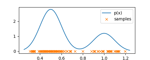
The above plot shows the observations/samples that we have access to. As I said before, histograms bin each dimension, so let’s bin the interval $[0.25, 1.25]$ in the plot above
delta = 0.1
bin_edges = np.arange(0.25, 1.25 + delta, delta)
ax.stem(bin_edges, [3 for _ in range(len(bin_edges))], markerfmt=' ', linefmt='k:', basefmt=' ')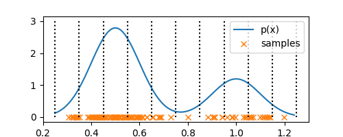
Each of these bins have a fixed volume of $\Delta = 0.1$. Now, all that is left is to determine $K$, a.k.a number of observations in each bin. Say, bin $i$ has $n_i$ observations in it, then we can compute probability density $p_i$ of the bin as
$$ p_i = \frac{n_i}{N\Delta} $$
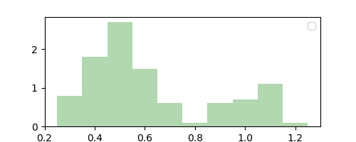
Thus, each bin has a probability mass of $p_i \Delta$ and summing the mass over all bins gives us $1$, as we would expect. Let’s see how this looks like in our $1$-D example:
histogram = np.array(
    [sum([x >= bin_edges[i] and x < bin_edges[i+1] for x in samples])
    for i in range(len(bin_edges)-1)]
)
normalized_histogram = (histogram / (N * delta))
plt.bar(bin_edges[:-1], normalized_histogram, align='edge', width=0.1, alpha=0.3, color='g')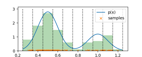
There you go! That’s it. We have our estimate for $p(x)$. Note that our estimate has constant density within each bin and has discontinuities across the bin edges. Keeping this aside, the estimate is a good representation of the underlying true density. Now that we have this estimate, we can throw away the observations and use this estimate from now on.
Our choice of $\Delta = 0.1$ was arbitrary and we could have chosen it to be anything. This is the distribution we get if we had chosen $\Delta = 0.01$.
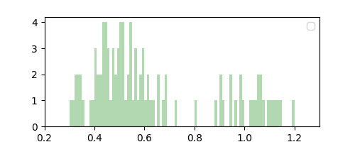
Observe that while $\Delta = 0.1$ resulted in a coarse smoothing estimate of $p(x)$, $\Delta = 0.01$ resulted in a finer but noisier estimate. Note that we did not compute this “parameter” from data, and instead it acts like a hyperparameter that can be chosen through domain knowledge or plain intuition. This makes the histogram method nonparametric.
Given our estimated density ($\Delta = 0.1$ histogram above,) we can now sample new observations from it (similar to image generation.) To do this, we first need to estimate the cumulative density function (CDF) as follows
estimated_pdf = lambda x: histogram[
    np.nonzero(np.logical_and(x >= bin_edges[:-1], x < bin_edges[1:]))[0][0]
]
estimated_cdf = np.cumsum([estimated_pdf(x) * delta * dx for x in xaxis])
plt.plot(xaxis, estimated_cdf, label="CDF estimate")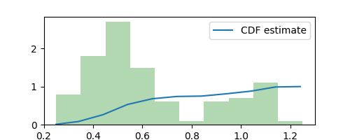
Now, we can just sample directly from our estimated distribution to generate new observations
M = 100
def sample_from_estimate():
    toss = np.random.rand()
    return xaxis[np.nonzero(estimated_cdf >= toss)[0][0]]

samples_from_estimate = [sample_from_estimate() for _ in range(M)]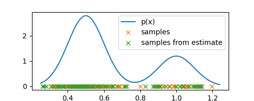
Note how the new observations/samples are concentrated around the regions where the old observations are, which means that our estimate is reasonably accurate and a good representation of the underlying density.
Empirical CDF
If estimating CDF was our only goal then, as someone on hacker news pointed out to me, we can achieve this in a much easier way by estimating the empirical CDF (ECDF) by simply assigning $1/N$ probability mass to each data point
X = sorted(samples)
Y = np.arange(N) / N
plt.step(X, Y, label="ECDF")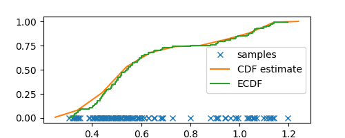
Observe how close our CDF estimate from histograms aligns with the empirical CDF, but more importantly, our histogram CDF estimate is smoother and less noisy. Furthermore, histograms also give us an estimate for the PDF that can be useful for estimating the density of any arbitrary sample (taking the derivative of ECDF can give us wild values.)
Why (not) Histograms?
Histograms are great at giving you a quick and easy visualization of your data, but it is mostly useful for 1- or 2-D problems. Unlike other nonparametric methods, histograms do not require us to store the observations, which is great if the data set is large and we have memory constraints.
As the dimensionality $D$ grows, the number of bins grows exponentially ($M$ bins in each dimension, results in a total of $M^D$ bins.) This exponential scaling makes histograms not the best for high-D density estimation, like realistic image generation. However, they are still a very useful tool to have in your arsenal.
In the next post, I will describe a very popular nonparametric method, Kernel Density Estimation, that also follows strategy 1 and is much more scalable to higher dimensions than histograms.
The source code for this post can be found here.