Very recently, I submitted a paper to RSS (update: accepted!) on how to use inaccurate models for planning in robotic tasks. For many robotic tasks, we usually have access to a (inaccurate) model of the robot and the environment. For example, simulators that employ sophisticated physics engines such as MuJoCo or Bullet can be used as forward dynamical models for planning. These models capture some complexities of the real world well, while they fail to capture other subtleties. However, they are still very useful sources of information on real-world dynamics that can be exploited to plan a good policy.
This paper from Abbeel, Quigley and Ng is one of my favourite papers in this domain. They have this really nice example and I quote
For example, if in a car our current policy drives a maneuver too far to the left, then driving in real-life will be what tells us that we are driving too far to the left. However, even a very poor model of the car can then be used to tell us that the change we should make is to turn the steering wheel clockwise (rather than anti-clockwise) to correct for this error.
This example perfectly summarises our motivation for this work. I strongly believe that not using an existing (inaccurate) model and purely using model-free approaches is like throwing out the baby with the bath water. If anything, using an existing model is a useful way to inject domain knowledge about the world into our approaches.
My paper is a small take on the following problem: Given an inaccurate dynamical model for a goal-oriented robotic task, how do we ensure that the robot provably reaches the goal online without any access to resets? Note that we tackle the no-reset setting as resets typically require human intervention, and this setting is more practical. We also consider deterministic dynamics and extension to stochastic dynamics is left open (potential future work.)
Let’s understand the problem through an example:
In the above video, we see a robot that is trying to move the light object from the start location to a goal location while avoiding collision with the obstacle. In this case, assume that we have access to a perfect dynamical model (true knowledge of the object weight, positions of obstacle etc.) With the perfect model, the planner comes up with an optimal path that takes the object above the obstacle and reaches the goal successfully. What if the object in reality was heavy, but is modeled as a light object?
It is not difficult to understand why the robot is stuck – since the model has not changed, the planner still computes the same path. But when the robot tries to follow the computed path it fails to lift the object beyond a certain height as the torque limits of the robot joints have been met and it cannot muster the required torque anymore. Thus, the robot (and the planner) is stuck. How do we solve this?
Most of the existing approaches tackle this by updating the dynamics of the model and replanning. Countless works along the lines of Dyna, and other model-based RL papers take this approach. However, with complex forward models (such as simulators, or analytical motion primitives among others) the dynamics cannot be changed arbitrarily online. These models tend to be inflexible and even in cases where they can be updated, it is a computationally expensive process that cannot be done online without sacrificing real-time capabilities. In addition, we also show that these approaches require a large number of online executions to reach the goal in our experiments.
Another set of works such as this paper and this one explore ideas of using residual dynamical models that are learned online to substantiate for the inaccuracies of existing models. However, these approaches are restricted heavily by the residual formulation (in most cases, its a simple additive correction on the next state.) Beside these two sets of approaches, the final set of approaches completely discard any existing model and try to learn a dynamical model from scratch (almost all of the current “deep” model-based approaches.) However, under our no-reset online setting they can take a really large number of samples before learning anything useful. More importantly, we care about reaching the goal quickly, and not on learning the true dynamics of the environment. In other words, we desire goal-oriented behavior in our approach.
Our approach uses the following key idea: Instead of learning the true dynamics online, CMAX maintains a running estimate of the set of transitions where the dynamics are inaccurate (we call these “incorrect” transitions,) and biases the planner to avoid these transitions in future replanning. The idea is very simple (some might say too simple) and we are not the first ones to discover it. It has often been used in practice as a hack! For instance, Zucker et. al. 2011 “poisoned” the cost function used by their footprint planner to ensure that the robot does not venture into poorly modeled terrain for their littleDog experiments. On the theoretical side, Jiang 2018 on PAC RL with imperfect models (Section 6) explored this idea in the discrete setting with access to resets. We extend this idea to the challenging no-reset setting and also present a practical algorithm for large (possibly, continuous) state spaces.
Penalized Model
We borrow the notion of penalized model from Jiang 2018. Given a deterministic shortest path problem $M = (\mathbb{S}, \mathbb{A}, \mathbb{G}, f, c)$ where $\mathbb{S}$ is the state space, $\mathbb{A}$ is the discrete action space, $\mathbb{G} \subset \mathbb{S}$ is the goal space, $f: \mathbb{S} \times \mathbb{A} \rightarrow \mathbb{S}$ is the unknown deterministic dynamics, and $c: \mathbb{S} \times \mathbb{A} \rightarrow [0, 1]$ is the cost function, we assume that we have access to an approximate model $\hat{f}: \mathbb{S} \times \mathbb{A} \rightarrow \mathbb{S}$ that is potentially inaccurate.
Given an “incorrect” set (set of incorrect transitions - transitions where $f$ and $\hat{f}$ differ) $\mathcal{X} \subset \mathbb{S} \times \mathbb{A}$, the penalized model is given as $M_\mathcal{X} = (\mathbb{S}, \mathbb{A}, \mathbb{G}, \hat{f}, c_{\mathcal{X}})$ where $c_\mathcal{X}(s, a) = c(s, a)$ for any $(s, a) \notin \mathcal{X}$, and $c(s, a) = |\mathbb{S}|$ (or any super large value) for $(s, a) \in \mathcal{X}$. In simple words, the cost of any transition known to be incorrect is inflated to a very high value. Thus, the name CMAX for our approach. We use the penalized model $M_\mathcal{X}$ for planning.
Warm Up: CMAX in small state spaces
Small state spaces are great! Planning is super fast and we can hope to plan all the way to the goal (has a complexity that scales with $|\mathbb{S}|$) In addition to fast planning, we can also maintain the set of incorrect transitions discovered so far $\mathcal{X}_t$ at each time step $t$ explicitly. This makes CMAX a very simple algorithm that is summarized as follows:
1. while s_t not in G:
2.    Get the best action a_t to execute at s_t by planning from s_t to any goal in G
3.    Execute a_t in the environment and get successor s_{t+1} = f(s_t, a_t)
4.    if s_{t+1} differs from successor predicted by penalized model:
5.        Update incorrect set X_{t+1} by adding (s_t, a_t) to X_t
6.        Update penalized model to M_{X_{t+1}}
It is important to note that we never update the dynamics of the model, only the cost function. For this simple algorithm, we can establish guarantees under the following assumption:
Assumption: There always exists a path from current state $s_t$ to a goal state that does not contain any transition that is known to be incorrect i.e. $(s, a) \in \mathcal{X}_t$
On close observation, we can deduce that this assumption is not as restrictive as the assumption that requires that there exists a path with only correct transitions. In other words, as long as the path does not contain a transition that is already discovered to be incorrect, the assumption is valid. This makes our assumption less restrictive, and our approach practically applicable. Under this assumption we have the following completeness guarantee:
Guarantee (Completeness): If initial value estimates are admissible (underestimates the optimal value at all states) and consistent (satisfies triangle inequality), then the robot is guaranteed to reach a goal state in at most $|\mathbb{S}|(|\mathcal{X}| + 1)$ time steps, where $\mathcal{X}$ is the set of all incorrect transitions.
In simple words, given enough time the robot is guaranteed to reach a goal! That is amazing and indicates that this approach is theoretically sound. However, to apply it in practice we need to move away from small state space land (Oh no!) to large state spaces, where
- we cannot plan all the way to the goal at every time step (too expensive!)
- we cannot maintain tabular value estimates for all states (too large!)
- we cannot maintain the incorrect set $\mathcal{X}_t$ so far explicitly (too large! slow lookup)
CMAX in large state spaces
We will deal with each of the above challenges individually. First, planning…
Limited-expansion search for planning
Limited expansion heuristic based search methods are often used for real-time planning applications where the amount of computation at each time step should not depend on the size of the state space. Popular examples include LRTA*, RTDP and RTAA* which have been successfully deployed in real-time applications.
We use a variant of RTAA* as the planner in CMAX for large state spaces. By using RTAA* with a fixed number $K < < |\mathbb{S}|$ expansions at each time step, we avoid expending computation of the order $O(|\mathbb{S}|)$ in each planning call. On a (very) high-level at each time step,
- we expand $K$ states to compute best action to execute for current state, and
- Update value estimates $V(s)$ for all expanded states.
The approach is summarized in the following figure (refer to the original paper for low-level details.)
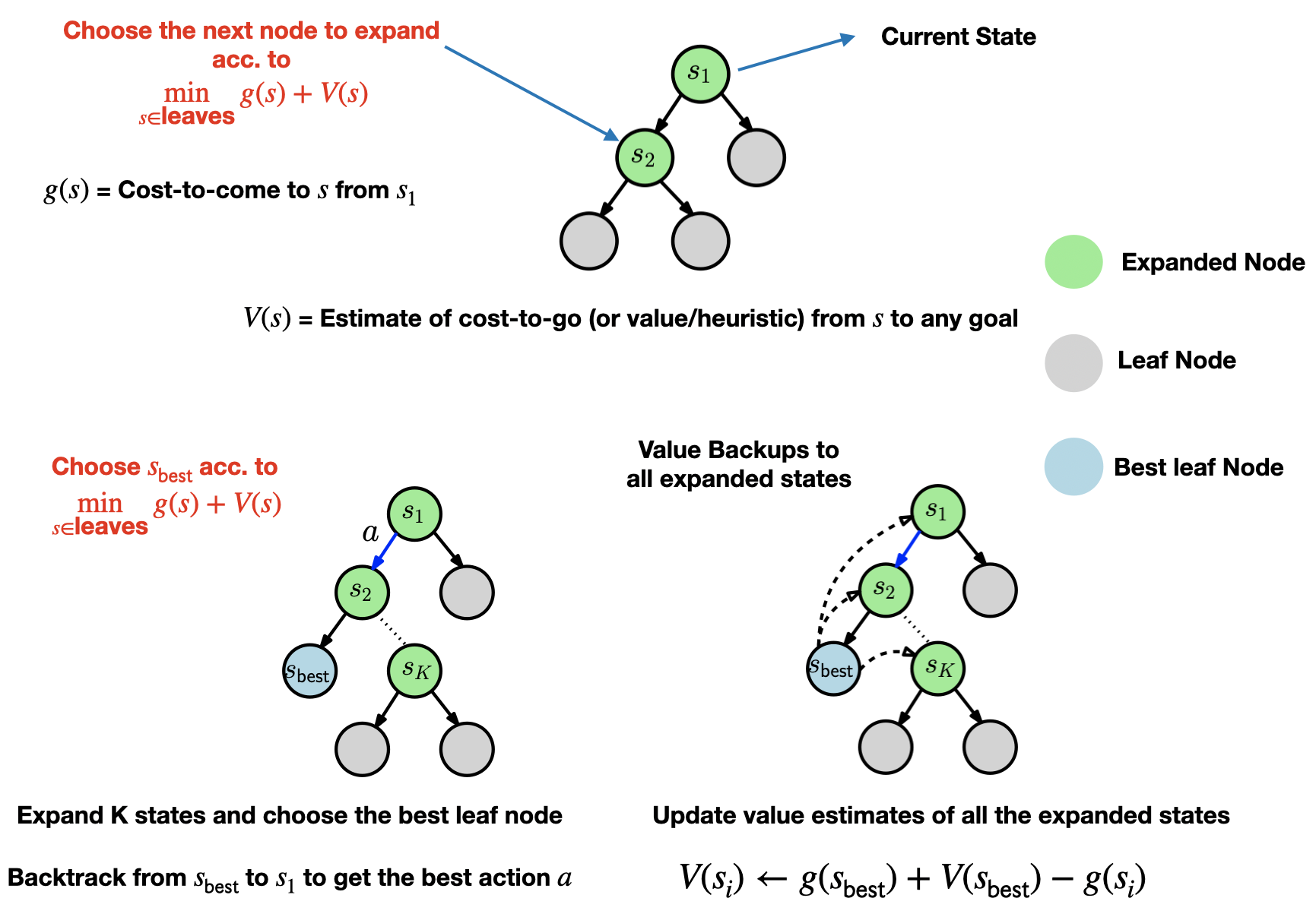
Fig. 1: Limited-expansion search as a planner. (Top) Leaves of the tree are expanded acc. to their g + V values. (Bottom left) After $K$ expansions, we choose the best leaf node acc. to the g + V value again. We backtrack from the best node all the way back to the start node to get the best action to execute at the start node (Bottom right) After figuring out the best action, we update the value estimates of all expanded states using the value estimate of the best node so that future replanning involving these states is more efficient.
However, by using a limited-expansion search as a planner the performance of CMAX heavily relies on the quality of value estimates. But in large state spaces, we cannot maintain tabular value estimates for all states and will have to resort to function approximation techniques.
Global Function Approximation for Value Estimates
Starting with the very popular DQN paper, there have been a very large number of works that have relied on global function approximation (e.g. neural networks) to maintain the value function in large state spaces. Although these techniques can make dynamic programming unstable in theory, they have shown amazing empirical performance. We borrow these ideas and use a neural network $V_\theta: \mathbb{S} \rightarrow \mathbb{R}$ parameterized by $\theta \in \mathbb{R}^n$ to maintain value estimates and perform approximate batch value updates:
$$\theta_{t+1} \leftarrow \theta_t - \frac{\eta}{2N} \nabla_\theta \sum_{i=1}^N (V_\theta(s_i) - (g(s_{best}) + V(s_{best}) - g(s_i))^2$$
where $\eta$ is the learning rate, and $\{s_i\}_{i=1}^N$ is a sampled mini-batch of states from a replay buffer. Crucially, unlike DQN we do not do one-step lookahead as we can simply use our approximate penalized model $M_{\mathcal{X}_t}$ to plan using $K$ expansions to get the target values $g(s_{best}) + V(s_{best}) - g(s_i)$ for each $i \in {1, \cdots, N}$. This speeds up fitting the value function approximation greatly as we backup value estimates from longer lookaheads.
Local Function Approximation for Incorrect Set $\mathcal{X}_t$
In large state spaces, the incorrect set $\mathcal{X}_t$ can be very large in size, and maintaining it explicitly can be expensive in both memory and computation during lookup. Thus, we need an efficient way to maintain it. CMAX achieves this by using local (or memory-based) function approximation using hyperspheres in state space. Specifically for every action $a \in \mathbb{A}$, we maintain a set of hyperspheres in state space $\mathbb{S}$ to represent $\mathcal{X}_t$.
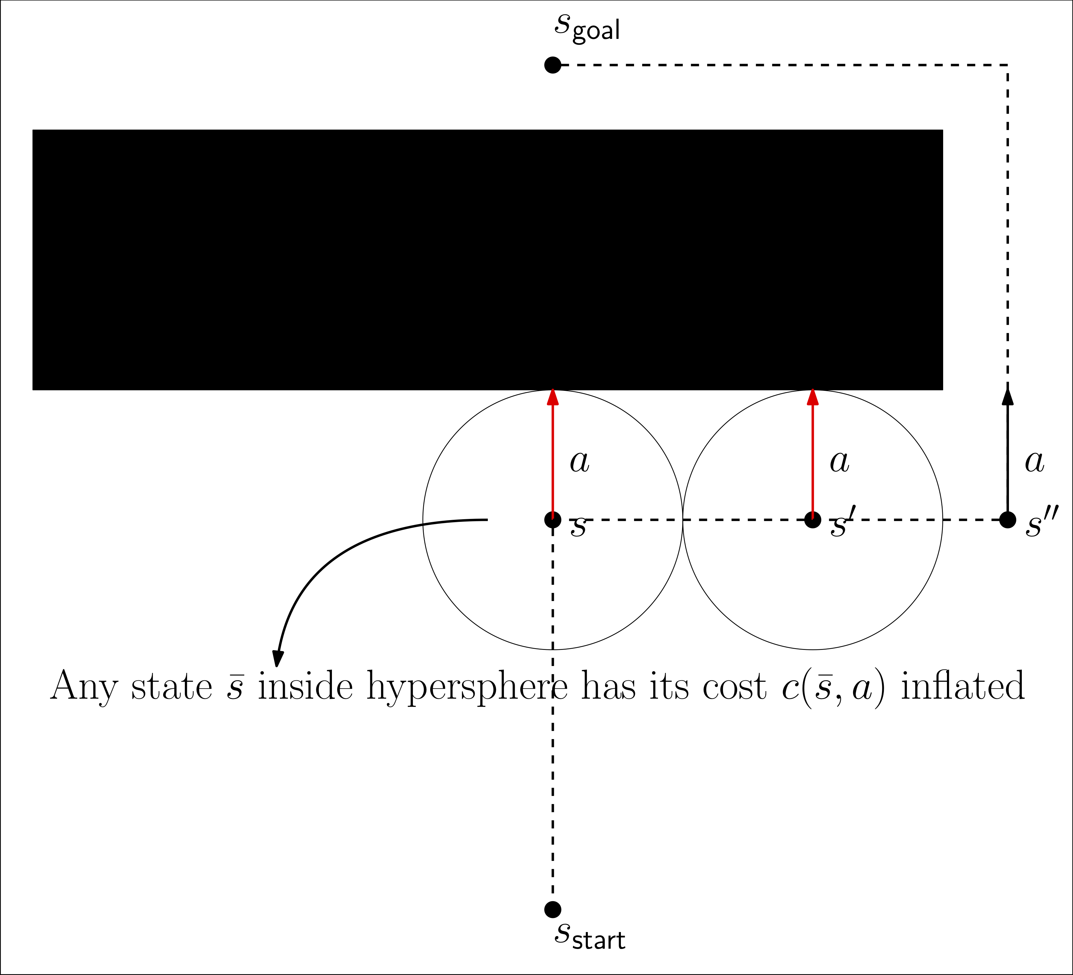
Fig. 2: Point robot navigation in the presence of obstacle. The dynamical model has no knowledge of the presence of the obstacle. During execution, any action that moves the robot into the obstacle keeps it in-place. The actions in red are incorrect transitions. Thus, we introduce hyperspheres at the corresponding states and the robot stops executing the action going into the obstacle until it gets out of the hypersphere, thereby reducing the number of steps taken to reach the goal.
During online execution, whenever we encounter an incorrect state-action pair $(s, a)$ a hypersphere of radius $\delta > 0$ centered at $s$. This hypersphere is added to the set of hyperspheres corresponding to action $a$. In any future replanning, any state-action pair $(\bar{s}, \bar{a})$ with $\bar{a} = a$ and $||\bar{s} - s||_2 \leq \delta$ has its cost inflated to a high value. The advantage of using hyperspheres is that lookup can be very efficiently implemented using KDTrees ($O(\log n)$ average complexity for lookup where $n$ is the number of hyperspheres.) Refer to Fig. 2 above for a simple example where we can quickly prune away the state space and find the path to the goal quickly. However, the radius $\delta$ is a very important parameter (that needs to be tuned – limitation of CMAX) since for small $\delta$ it might take a large number of online executions to reach the goal, and for large $\delta$ it might block the only path to the goal which can be disastrous.
Summary
Let’s summarize the key ideas in CMAX:
- Inflate the cost of any incorrect transition discovered to bias planner away from using these transitions in future replanning
- Use limited-expansion search as the planner to limit amount of computation at each time step. Thus, it can be used in large state spaces
- Employ global function approximation techniques to maintain value estimates for all states
- Maintain incorrect set $\mathcal{X}_t$ using local function approximation in state space
Experiments
Going back to our motivating example of a 3D pick-and-place task with a heavy object, let us see how CMAX performs:
Upon recognizing the discrepancy in dynamics between the model and the environment, CMAX (instead of learning the true dynamics and correcting the model) quickly adapts and finds an alternative path that takes the object behind the obstacle to the goal. This kind of highly goal-oriented behavior at the expense of less number of executions is exactly the behavior we want.
We also test CMAX in large state spaces in our 7D arm planning task where the objective is to move the 7D arm from a start configuration to a goal configuration such that its end effector is within a specified 3D goal region. However, the catch is that one of its joint is broken, and it has to still find a path to the goal despite the inaccuracy of the model.
Again, CMAX quickly “covers” the state-action space that is modeled incorrectly with hyperspheres, to find a path that uses the unbroken joints to move the end-effector to the goal region.
For a quantitative comparison, we compare the number of time steps it takes for CMAX to reach the goal against baselines that are both model-based (updating residual model and replanning), and model-free. Specifically, we compare CMAX against the baselines on a 4D simulated planar pushing task.
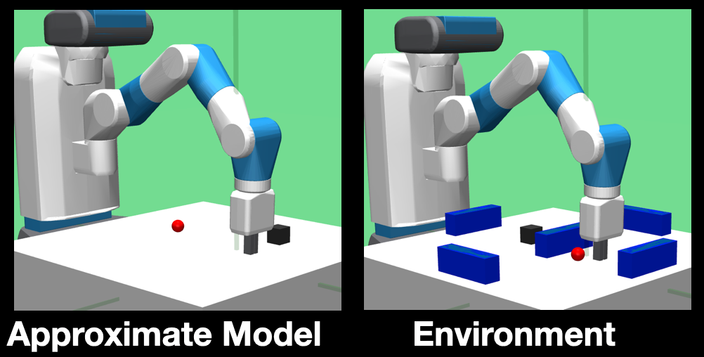
Fig. 3: 4D simulated planar pushing. (left) The approximate model available for planning that does not contain any obstacles so the robot has to discover the obstacles through online executions in the environment (right) which contains obstacles. The goal for the gripper is to push the object (black box) from its current position to the goal location (red sphere). When the gripper (or) the object is pushed into an obstacle, they stay in place.
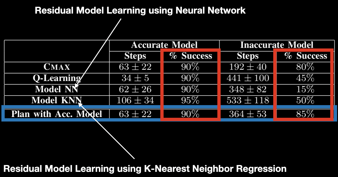
Fig. 4: 4D planar pushing results. The first column is the number of time steps it takes to reach the goal when planning and executing in the environment with no obstacles. The second column is the number of time steps it takes to reach the goal when planning using the model with no obstacles and executing in environment with obstacles. Success rate is computed using the ratio of successful runs where a run is successful if the object reaches the goal in under 1000 time steps.
Discussion
CMAX achieves all of this while never attempting to learn the true dynamics! And the true strength of CMAX lies in that. This can be better understood by a simple argument: to learn accurate dynamics for a transition in $N$-D state space we need at least $N$ samples in worst case, whereas CMAX needs only $1$ sample to observe a discrepancy and inflate the cost. CMAX also can be applied to problems where the approximate model is inflexible and cannot be updated arbitrarily online (think of complex physics engines). It does not rely on any knowledge of how the approximate model is inaccurate. Finally, in the extreme case where we can never hope to learn the true dynamics using any sort of function approximation (think of deformable object dynamics,) CMAX can still be applied!
However, we do not get all of these advantages for free. The crucial assumption that there always exists a path with no transitions that are known to be incorrect, or model optimism as Jiang 2018 calls it, is essential. Apart from the tuning of radius $\delta$, this assumption is the biggest limitation of CMAX. One can easily come up with robotic tasks where this assumption is violated : for instance, consider the task of opening a spring loaded door which is not modeled as spring loaded, we would notice discrepancy in every transition and the assumption is not valid anymore. However, I still believe that CMAX is very useful in a lot of practical scenarios (as our experiments show) and it is a very easy-to-implement baseline that everyone should compare against.
Epilogue
(May 15 2020) Few clarifications are in order regarding the assumption presented above (Thanks to Alex Spitzer for the questions.) A keen observer would notice that the assumption, as it is presented, is actually an assumption on both the approximate dynamical model $\hat{f}$ and the execution trace of CMAX (since the assumption is conditioned on the current state $s_t$.) This can be a little confusing since such an assumption is hard to verify prior to execution and unfortunately, that is indeed the case here. However, we can strengthen the assumption in the small state cases using the model optimism assumption from Jiang 2018. Specifically, an optimistic dynamical model is a model whose optimal value under approximate dynamics $\hat{f}$ at each state $s \in \mathbb{S}$ underestimates the optimal value under true dynamics $f$. In small state cases where we can afford to plan all the way to the goal at each time step and obtain the best action, model optimism is a sufficient assumption to ensure the above completeness guarantee. Put simply, if our approximate dynamical model is optimistic we will never encounter states where the above assumption is invalid. However, it gets complicated in large state spaces (as things often do.) Since we perform limited-expansion search with potentially suboptimal value estimates (and thus, there is no guarantee that we execute the best action,) model optimism is not sufficient anymore and we require the assumption on the execution trace of CMAX.
(May 25 2020) Arvind Rajeswaran, Rahul Kidambi and collaborators have recently released a paper that has very similar ideas to CMAX and Jiang 2018, but in the offline RL setting. They also propose construction of a “pessimistic” MDP from offline trajectories which divides the state-action space into a “known” (correct) and “unknown” (incorrect) region. Subsequently, they plan for a policy in the pessimistic MDP that enters into a low reward (high cost) absorbing state upon executing an “unknown” transition. Thus, the policy learns to stay in the “known” region and exhibit CMAX-like behavior. The paper also presents bounds on the performance of the optimal policy obtained from planning in the pessimistic MDP under idealistic assumptions. Another very recent work from Tianhe Yu and collaborators from Stanford presents a very similar idea, again in the offline RL setting. Rather than a hard penalty for state-action pairs in the unknown region, they apply a soft penalty based on how large an estimate of the modeling error is. From a pure planning perspective (like CMAX,) Dale McConcachie and collaborators have also recently used a very similar idea to bias the planner away from incorrect transitions. However, unlike CMAX, during online execution they employ a offline trained classifier to predict whether any transition is incorrect, thus relying on the accuracy of the trained classifier to ensure probabilistic completeness.
CMAX and all of the above works indicate that we can achieve impressive practical results with good theoretical foundation for model-based planning with imperfect models. I am hopeful that the community takes this forward and develops algorithms that relax some of the assumptions made by these works.