A Gentle Primer for Nonparametric Density Estimation: Kernel Density Estimation

In my previous post, we discussed a neat intuition for nonparametric density estimation and introduced a nonparametric method, histograms. This post describes another (very popular) density estimation method called Kernel Density Estimation (KDE).

Revisit Intuition

Let’s revisit the intuition that we developed for nonparametric density estimation. Given a region $R \subset \mathbb{R}^D$ of volume $V$, and that contains $K$ points from a sampled dataset of size $N$, we can estimate $p(x)$ for any point $x \in R$ as

$$ p(x) = \frac{K}{NV} $$

We have shown that this intuition lends us two strategies for estimating $p(x)$:

1. We can fix $V$ and determine $K$ from data
2. We can fix $K$ and determine $V$ from data

Histograms, as described in the previous post, use strategy 1 where we fix the bin volume and determine how many points fall within each bin from the data. Kernel Density Estimation, as we will see, follows the same strategy with two major differences:

1. Regions $R$ (or the bins) are centered on data points
2. Use of kernel functions to represent density in region $R$

Kernel Density Estimation

Extending the binning idea of histograms, let’s take the region $R$ to be a small hypercube of side $\Delta$ centered at any $x \in \mathbb{R}^D$. Note that in histograms, the regions were always centered at the discretization of $\mathbb{R}^D$ space.

Using the same 1-D example as the previous post we can visualize how this hypercube would look like at an arbitrary $x$

delta = 0.1
x = 1.0
ax.stem([x - delta/2, x + delta/2], [3, 3], markerfmt=' ', linefmt='k:', basefmt=' ')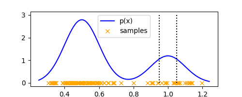

Looks exactly like a histogram bin, except it is defined at any arbitrary $x$ (and not the discretization points, like in histogram.) To count the number of points ($K$) falling within $R$, we can define the function $k(u)$,

$$ k(u) = \begin{cases} 1, & \text{if } |u_i| \leq \frac{1}{2}, \forall i=1,\cdots,D \\ 0, & \text{otherwise} \end{cases} $$

We can now count the number of points $K$ within $R$ by noting that the quantity $k(\frac{x - x_n}{\Delta})$ is $1$ if data point $x_n$ is inside the hypercube $R$ and $0$ otherwise.

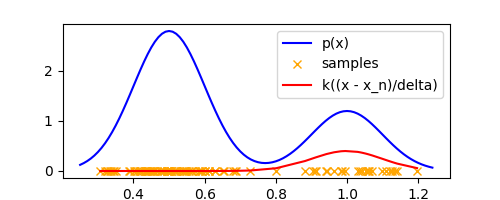
Let’s plot $k(\frac{x - x_n}{\Delta})$ for all samples $x_n$ in the above example,

k = lambda u: 1 if abs(u) <= 0.5 else 0
sorted_samples = sorted(samples)
plt.plot(
    sorted_samples, 
    [k((x_n - x) / delta) for x_n in sorted_samples], 
    label='k((x - x_n)/delta)', 
    color='red'
)

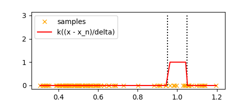
Looks like a box, doesn’t it? Now we can simply count the number of points $K$ inside this box to estimate the density at $x$. Thus, we can estimate $K$ as

$$ K = \sum_{i=1}^N k\left(\frac{x - x_n}{\Delta}\right) $$

Substituting the above equation into the nonparametric density estimation intuition equation, we get

$$ p(x) = \frac{1}{N\Delta^D} \sum_{i=1}^N k\left(\frac{x - x_n}{\Delta}\right) $$

where we used the fact that the volume of the $D$-dimensional hypercube of side $\Delta$ is $V = \Delta^D$. Let’s plot $p(x)$ for our 1-D example,

K = lambda x: sum([k((x - x_n) / delta) for x_n in samples])
p = lambda x: K(x) / (N * delta)
plt.plot(xaxis, list(map(p, xaxis)), label="p(x) estimate", color='red')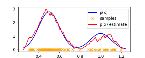

Not a bad estimate! Looks a little noisy but approximates the true density quite well.

However, the interpretation of placing a region at every point $x$ and counting number of points in the region sounds cumbersome. We can use a symmetry argument by noting that our function $k$ is symmetric (i.e. $k(u) = k(-u)$) to reinterpret our density estimate, not as a single hypercube centered at $x$ but as the sum over $N$ cubes centered on each of the $N$ data points $x_n$!

Thus, so far, the only difference from histograms was that the bin centers are on the data points themselves! As a result of this, the bins can overlap and we compute the density estimate at $x$ as the sum of density estimates from all overlapping bins. This eliminates the need to discretize the input space, as needed in histograms, and gives us a more smooth (and less discrete) density estimate than histograms.

Kernel Functions

The density estimate from the above plot still looks “choppy” (its actually discontinuous and they would be visible at inifinitesimally small resolution.) This is because, the density estimate “jumps” at the hypercube boundaries as the “influence” of a data point on the estimate begins/terminates.

We can fix this by changing the function $k(u)$ that we used. $k(u)$ is an example of a kernel function, specifically a box kernel. We can choose any kernel function $k(u)$ to ensure that the resulting estimate is a valid probability distribution as long as,

$$ k(u) \geq 0 $$

$$ \int k(u) du = 1 $$

To avoid the discontinuities, we can choose a smoother kernel function that has “soft” boundaries, such as a Gaussian kernel

$$ k(u) = \frac{1}{(2\pi)^{\frac{D}{2}}} \exp\left(-\frac{||u||^2}{2}\right) $$

Let’s plot $k(\frac{x - x_n}{\Delta})$ for all samples $x_n$ in our 1-D example at a specific $x$ and visualize it

x = 1.0
gaussian_k = lambda u: (1/(2*math.pi)**0.5) * math.exp(-0.5 * u**2)
plt.plot(
    sorted_samples,
    [gaussian_k((x_n - x) / delta) for x_n in sorted_samples],
    label='k((x - x_n)/delta)', 
    color='red'
)

K = lambda x: sum([gaussian_k((x - x_n) / delta) for x_n in samples])
p = lambda x: K(x) / (N * delta)
plt.plot(xaxis, list(map(p, xaxis)), label="p(x) estimate", color='red')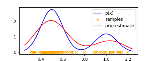

Voila! We have a smooth estimate of the density function that approximates the underlying density reasonably well. Thus, our density model is obtained by placing a Gaussian over each of the $N$ data points, adding up their contributions over the entire dataset, and dividing by $N$ to get a normalized density estimate.

We can make the approximation more accurate by tweaking $\Delta$, which in the context of a Gaussian kernel is the variance of the kernel. Using $\Delta = 0.05$, we get the following plot which already looks very much like the true density

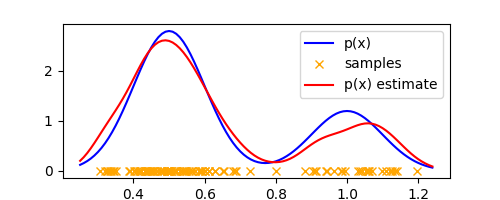
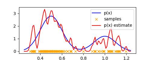
We see that similar to histograms, $\Delta$ plays the role of a smoothing parameter and we obtain over-smoothing for large values of $\Delta$ and sensitivity to noise in the dataset for small values. Thus, the parameter $\Delta$ controls the complexity of the density model. As an example, here’s the estimate with $\Delta = 0.01$ that shows sensitivity to noise.

And that’s Kernel Density Estimation. The only differences from histogram were:

1. Using regions centered on data points
2. Flexibility to use any kernel function to represent the density in a region

Interested readers can check out this super cool interactive blog post that allows you to play with different kernel functions and different values of $\Delta$ to visualize resulting density estimates and the influence of data points on the estimate.

Why (not) Kernel Density Estimation?

Similar to histograms, KDE is a nonparametric method that does not compute any parameters from data. While our post has explored two kernel functions: box and Gaussian kernel, there are a lot of kernel functions, and using them gives user a wide range of modeling choices that is not available with histograms.

The greatest merit of KDE over histograms is that it scales well to higher dimensional density estimation, as the number of “regions” do not scale exponentially in input dimension, unlike histograms. Furthermore, there is virtually no computation involved in the “training” phase for KDE as we simply require the training data to be stored to be used at inference time.

However, this means that the computational complexity (and the number of “regions”) of KDE scales linearly with the data size, which makes it prohibitive to use for large datasets. This is compounded in high dimensions, where we require a large number of data points to reliably estimate the density, making KDE computationally more expensive as a result.

In the next post, we will finally introduce a nonparametric method that follows strategy 2, nearest neighbors density estimation, where we fix $K$ and estimate $V$ from data.

The source code for this post can be found here.