In this blog post, I will summarize the key contributions of my recent submission on CMAX++. This work mainly improves upon my previous work, CMAX (highly recommended to read a summary of CMAX in this blog post.)
The broad theme of both these approaches is to use simplified and inaccurate dynamical models to significantly reduce the amount of real world experience needed by the robot to complete a task. The setting we consider is a goal-oriented task setting where the robot needs to reach the goal online, without any resets. This setting is classically considered using the planning and execution framework where the robot constantly replans after each execution to intelligently use any experience obtained in the past executions. It goes without saying that this setting is extremely challenging as the initial model used for planning cannot capture the real world dynamics accurately and the robot does not have access to any resets to “undo” any past mistakes.
In addition in this work, we primarily deal with repetitive robotic tasks where we require the robot to complete the task in each repetition and expect to improve its task performance across repetitions.
Examples
Let us understand the problem through an example (this is very similar to the motivating example used in CMAX):
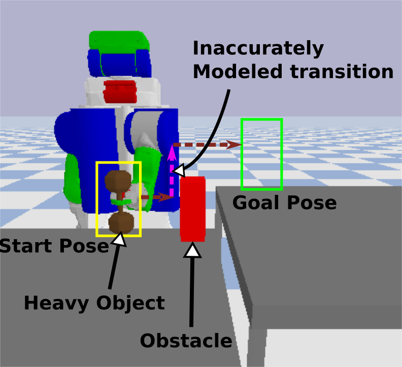
Fig. 1: PR2 lifting a heavy dumbbell, that is modeled as light, to a goal location that is higher than the start location resulting in dynamics that are inaccurately modeled. Note that any path to the goal requires executing an inaccurately modeled transition (pink.)
In the above figure, PR2 is lifting a heavy object (modeled as light) from a start pose to a goal pose (goal is on a higher table than start) while avoiding collision with the obstacle. Note that since the goal location is higher than start, the robot has to lift the object higher if it wants to reach the goal. Since the object is heavy, the robot cannot generate required forces in certain arm configurations and can only lift the object to smaller heights. Let us understand how CMAX works in this task as the robot repeatedly picks the object at the start and places it at goal. CMAX inflates the cost of any transition that lifts the object higher as the dynamics are inaccurately modeled. This results in plans that avoid lifting the object in future repetitions. Thus, the quality of CMAX solution deteriorates across repetitions, and in some cases, it even fails to complete the task. Although, CMAX reaches the goal quickly in a goal-driven fashion in the first repetition, it can be highly suboptimal in later repetitions.
We will emphasize this using another example:
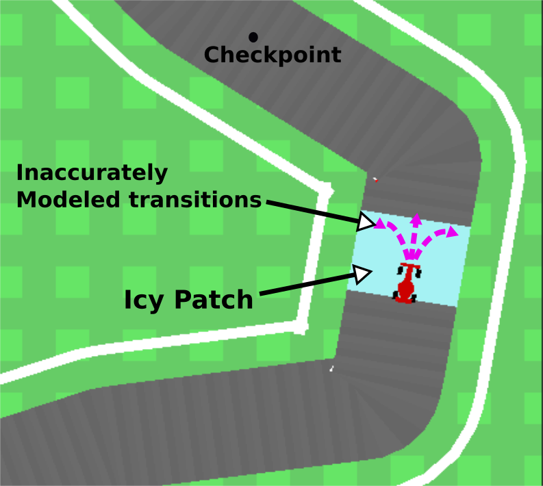
Fig. 2: Mobile robot navigating around a track with icy patches that have unknown friction parameters leading to the robot skidding. Any path that takes the robot to the checkpoint requires executing an inaccurately modeled transition (pink.)
Objectives and Problem Formulation
Our objective in this work is two-fold:
- Provably reach goal online in each repetition, despite using an inaccurate model, without any resets allowing the path to contain inaccurately modeled transitions
- Leverage experience from past executions to improve task performance across repetitions
We formulate this as a shortest path problem $M = (\mathbb{S}, \mathbb{A}, \mathbb{G}, f, c)$ where $\mathbb{S}$ is the state space, $\mathbb{A}$ is the discrete action space, $\mathbb{G} \subset \mathbb{S}$ is the goal space, $f:\mathbb{S}\times\mathbb{A}\rightarrow\mathbb{S}$ is the true unknown deterministic dynamics, and $c:\mathbb{S}\times\mathbb{A}\rightarrow [0, 1]$ is the cost function. We assume that we have access to an approximate model $\hat{f}:\mathbb{S}\times\mathbb{A}\rightarrow\mathbb{S}$ that is potentially inaccurate. We call a transition $(s, a)$ as “incorrect” if the true dynamics $f$ and approximate dynamics $\hat{f}$ differ on $(s, a)$. This notion of “incorrectness” is task-specific and is usually set to a threshold that reflects the maximum discrepancy that a low-level path following controller (such as a PID or any feedback controller) can substantiate for. See the paper for more details.
Existing Work
We highlight existing work that tackles related problems in the following figure:
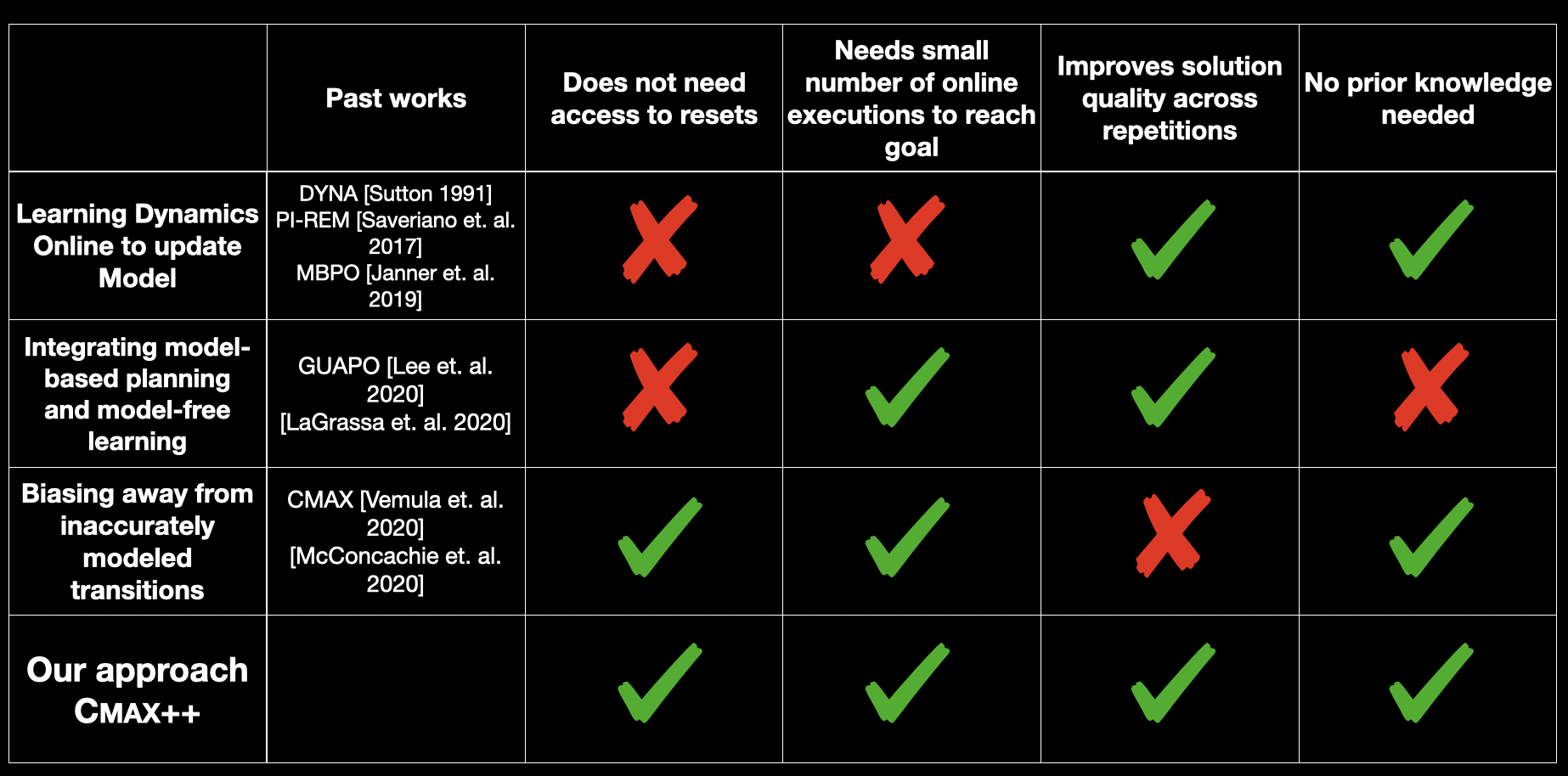
Fig. 3: Related Work and their pros/cons
The first set of works (first row in the above figure) are approaches that use the acquired experience through executions to update dynamics of the approximate model. While this is the predominant approach in modern model-based RL literature, it is extremely sample-inefficient especially when you have no access to resets. However, these approaches tend to improve the performance of their solution as the amount of acquired experience grows and require no prior knowledge on how the initial model was inaccurate.
The second set of works are more recent and are similar to our approach CMAX++ in the way they integrate model-free learning with model-based planning. While they are usually sample-efficient, existing approaches require access to resets and prior knowledge on how/where the initial approximate model is inaccurate or require access to expert demonstrations.
The last set of works are very similar to CMAX and deal with inaccurate models by adapting the behavior of the planner to bias away from inaccurately modeled regions. These methods tend to be highly sample-efficient, do not require resets and no prior knowledge is needed. But as illustrated in our examples above, these methods lack the property of improving task performance as the amount of acquired experience grows.
In contrast to all these approaches, our approach CMAX++ does not need access to resets or prior knowledge while improving task performance across repetitions and requiring limited amount of real world experience.
CMAX++
Key Idea
Maintain model-free Q-value estimates of incorrect transitions and integrate them into model-based planning using the inaccurate model
Unlike previous approaches that used experience to either update model dynamics or to inflate cost of incorrect transitions, CMAX++ simply learns a model-free Q-value estimate for these transitions. The Q-value for any transition $(s, a)$ captures the future cost-to-go incurred to reach a goal after executing transition $(s, a)$.
CMAX++ is summarized in the following figure:
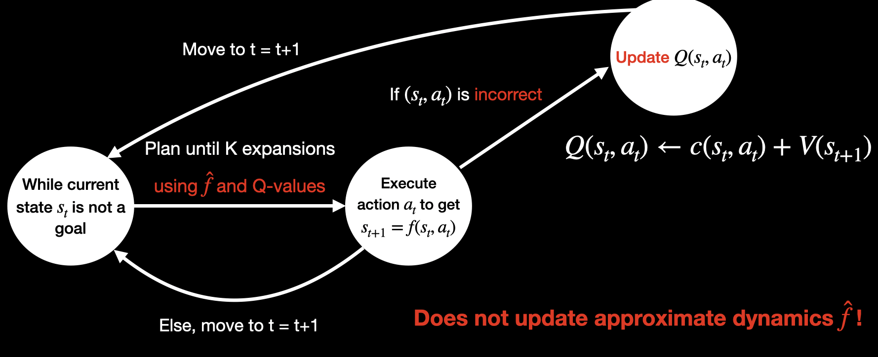
While the current state $s_t$ is not a goal, we plan (more on this later) using the inaccurate model $\hat{f}$ and Q-values estimated so far to get the best action to execute $a_t$. This action is executed in the real world to get the true successor $s_{t+1} = f(s_t, a_t)$. If $(s_t, a_t)$ is incorrect (i.e. $s_{t+1}$ and $\hat{f}(s_t, a_t)$ differ) then we estimate the Q-value $Q(s_t, a_t) \leftarrow c(s_t, a_t) + V(s_{t+1})$ and store it. Subsequently (or if $(s_t, a_t)$ was not found to be incorrect,) we simply replan from the new state. This process is repeated until we reach a goal.
It is very important to note that CMAX++, instead of storing the true successor $s_{t+1}$, only estimates and stores the model-free Q-value $Q(s_t, a_t)$ and thus never updates dynamics of the approximate model.
One of the key contributions in our work is integrating these model-free Q-value estimates into a model-based planning procedure which is explained below.
Integrating Q-values into Model-based Planning
For planning, we use a limited expansion search-based planner. Please refer to this section of the CMAX blog post for a quick refresher. We use a limited expansion search-based planner as it intuitively accommodates including Q-values into the search tree constructed at the current state $s_t$. This section is a very quick and concise description of the planner and for more details, you should check out our paper.
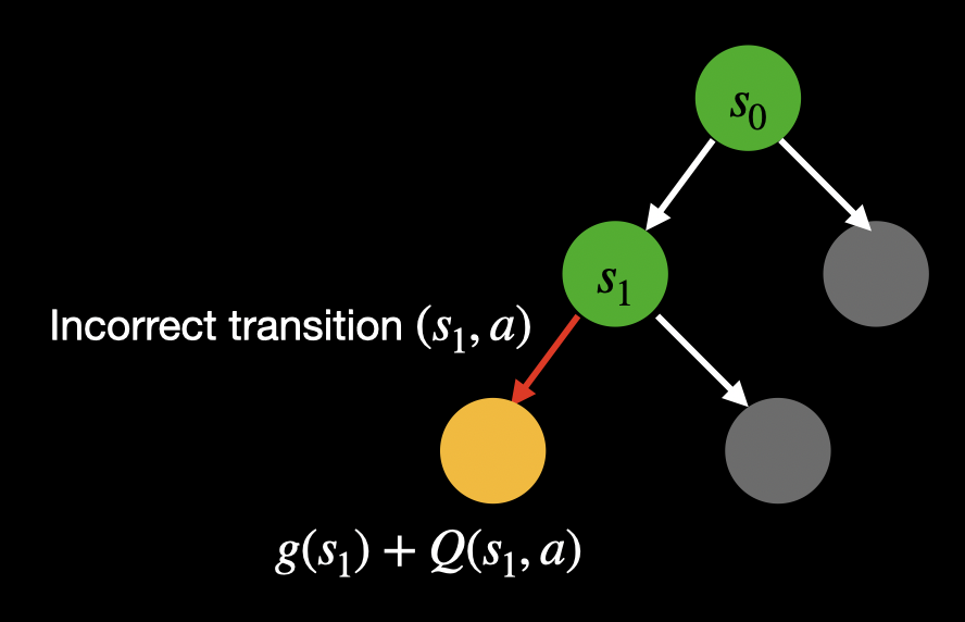
During the search-tree construction, if we ever encounter an incorrect transition then we add a dummy state as the child node because we are unaware of its true successor (remember, we only update Q-value estimate upon execution of incorrect transition and not update dynamics or store successor.) To integrate this dummy state into the search procedure, we need to estimate its priority. In heuristic-based search, the priority of any state/node $s$ is estimated as $g(s) + V(s)$ where $g(s)$ is the cost-to-come to $s$ from the root of the tree, and $V(s)$ is the cost-to-go incurred from $s$ to a goal.
But we cannot estimate $V(s)$ for this dummy state as we do not know what state it truly corresponds to. CMAX++ resolves this by instead using the estimated model-free Q-value of the incorrect transition the dummy state corresponds to. In other words, we compute the priority of the dummy state which is created as a successor of incorrect transition $(s, a)$ as $g(s) + Q(s, a)$. This is summarized in the figure below.
Finally, if the dummy state is chosen as the next node to be expanded (the leaf node with the least priority is always chosen to be the next node to be expanded) then we terminate the search as we are unaware of the true state it corresponds to. In such a case, the dummy state is chosen as the best node and we backtrack from it to the root to find the best action $a_t$ to execute at the root. We also use the best node to update the value estimates of all expanded states as $V(s_{\mathsf{expanded}}) \leftarrow p(s_{\mathsf{best}}) - g(s_{\mathsf{expanded}})$ where $p(s_{\mathsf{best}})$ is the priority of the best node.
Note that our hybrid planner can return plans that contain incorrect transitions (especially if they have low Q-values) and can propagate model-free Q-value estimates using model-based planning. Both of these attributes are very important reasons for why CMAX++ works so well in practice.
Limitation of CMAX++
We now have a planning approach, CMAX++, that can utilize previously discovered incorrect transitions if they lead to a goal with low cost. However, naively using CMAX++ in practice will lead to a large number of online executions wasted to learn accurate model-free Q-value estimates. This is a well-studied phenomenon where model-free approaches are known to be less sample-efficient when compared to model-based procedures. See this paper and this paper.
Put simply, while CMAX++ can discover paths to goals that can potentially use incorrect transitions, it takes a large number of executions to realize the usefulness of these transitions. In such situations, it might simply be better to stick to regions where the model is accurate (so that we can do the more efficient planning procedures) and find an alternative path. This is exactly what CMAX does! So, is there a way to get the best of CMAX’s goal-driven behavior and CMAX++’s optimal behavior while ensuring that we do not waste online executions and reach the goal in each repetition?
Turns out we can :)
Adaptive-CMAX++
Key Idea
Intelligently switch between CMAX and CMAX++ during execution to combine the advantages of both
The above idea is implemented by maintaining two sets of value estimates:
- Non-Penalized Value Estimates: $V$ obtained from planning using CMAX++ without inflating costs and instead using model-free Q-value estimates for incorrect transitions
- Penalized Value Estimates: $\tilde{V}$ obtained from planning using CMAX by inflating the costs of incorrect transitions
With the above two sets of value estimates, and a sequence $\alpha_1, \cdots, \alpha_N$ where $N$ is the total number of repetitions such that $\alpha_1 \geq \alpha_2 \geq \cdots \geq \alpha_N \geq 1$, Adaptive-CMAX++ works as follows: At each time step $t$ in repetition $i$, if $\tilde{V}(s_t) \leq \alpha_i V(s_t)$, execute CMAX action or else, execute CMAX++ action.
In words, if the cost-to-go incurred by following CMAX in future is within $\alpha_i$ times the cost-to-go incurred by following CMAX++, then we prefer CMAX. Else, we prefer CMAX++.
This induces a goal-driven behavior (by virtue of picking CMAX actions) in early repetitions when $\alpha_i$ is large, and optimal behavior (by virtue of picking CMAX++ actions) in later repetitions when $\alpha_i$ is small.
Furthermore, the large number of executions needed by CMAX++ to learn accurate Q-value estimates is distributed across repetitions ensuring that Adaptive-CMAX++ does not have poor performance in any single repetition.
Theoretical Guarantees
We will show that CMAX++ has the same guarantees as CMAX under much weaker conditions. In addition, CMAX++ also has an asymptotic convergence guarantee that ensures that the task performance improves across repetitions.
Firstly, let us state the optimistic-model assumption that was first introduced in Jiang 2018 that is needed by CMAX++ and Adaptive-CMAX++.
Optimistic Model Assumption: Optimal value function $\hat{V}^* $ under the approximate dynamics $\hat{f}$ underestimates the optimal value function $V^*$ under true dynamics $f$ at all states, i.e. $\hat{V}^*(s) \leq V^*(s)$
Intuitively, this means that the robot using the approximate dynamics should never be “pleasantly surprised” by what it observes in the environment. I like to think of it in the following way: the model should never predict there is an obstacle where there isn’t any, while it can always predict that there is no obstacle when there truly is an obstacle.
It is very easy to see that this assumption is much more relaxed when compared to CMAX assumption (which basically amounts to having an optimistic model under the penalized cost function at all time steps during execution.)
Completeness Guarantee: Under the optimistic model assumption (or CMAX assumption,) a robot using CMAX++ or Adaptive-CMAX++ is guaranteed to reach a goal in each repetition in atmost $|\mathbb{S}|^3$ time steps. Furthermore, if CMAX assumption holds and if $\alpha_i$ for repetition $i$ is sufficiently large, then Adaptive-CMAX++ is guaranteed to reach a goal in atmost $|\mathbb{S}|^2$ time steps.
The above guarantee simply claims that the robot is guaranteed to reach the goal in each repetition. Under the much stronger CMAX assumption, the guarantee also shows a gap between the worst case bound between CMAX++ and Adaptive-CMAX++ highlighting cases when Adaptive-CMAX++ can reach the goal quicker than CMAX++.
Asymptotic Guarantee: Under the optimistic model assumption, both CMAX++ and Adaptive-CMAX++ are guaranteed to converge to the path with optimal cost as number of repetitions grow.
This guarantee states that as the amount of acquired experience grows, CMAX++ and Adaptive-CMAX++ converge to optimal paths to the goal. This is unlike CMAX, where the experience is only used to bias the planner away resulting in suboptimal paths to the goal.
Thus, we have provable guarantees that CMAX++ (and Adaptive-CMAX++) achieve the objectives we started out with.
CMAX++ in Large State Spaces
CMAX++ (and Adaptive-CMAX++) can be extended to work in large state spaces where we cannot have tabular representation to maintain value estimates (both $V$ and $Q$) and we cannot explicitly store all the incorrect transitions. We use the same tricks that CMAX employs, so I will refrain from repeating here and simply refer the reader to the appropriate part of the CMAX blog post.
Summary
We unpacked a lot of stuff so far. It is useful to summarize the key contributions:
- Instead of inflating cost, learn model-free Q-value estimates of incorrect transitions from experience
- Integrate learned model-free Q-value estimates into model-based planning procedure with inaccurate model
- Intelligently switch between CMAX++ and CMAX during execution to combine goal-driven behavior and optimal behavior
- Use function approximation techniques to scale Adaptive-CMAX++ and CMAX++ to large state spaces
Experiments
Going back to our motivating example of 3D mobile robot navigation with icy patches, let us see how CMAX++ and Adaptive-CMAX++ perform against CMAX. The objective of the task is to finish $200$ laps around the track with icy patches. The approximate model used by the robot does not have icy patches and hence does not accurately model any transition within the icy patch that results in the robot skidding. This is formulated as a planning problem with a small 3D discrete state space $(x, y, \theta)$ and the action space is a discrete set of pre-computed motion primitives that respects the differential drive dynamics of the robot. For more details on motion primitives and lattice graphs, refer to this paper.
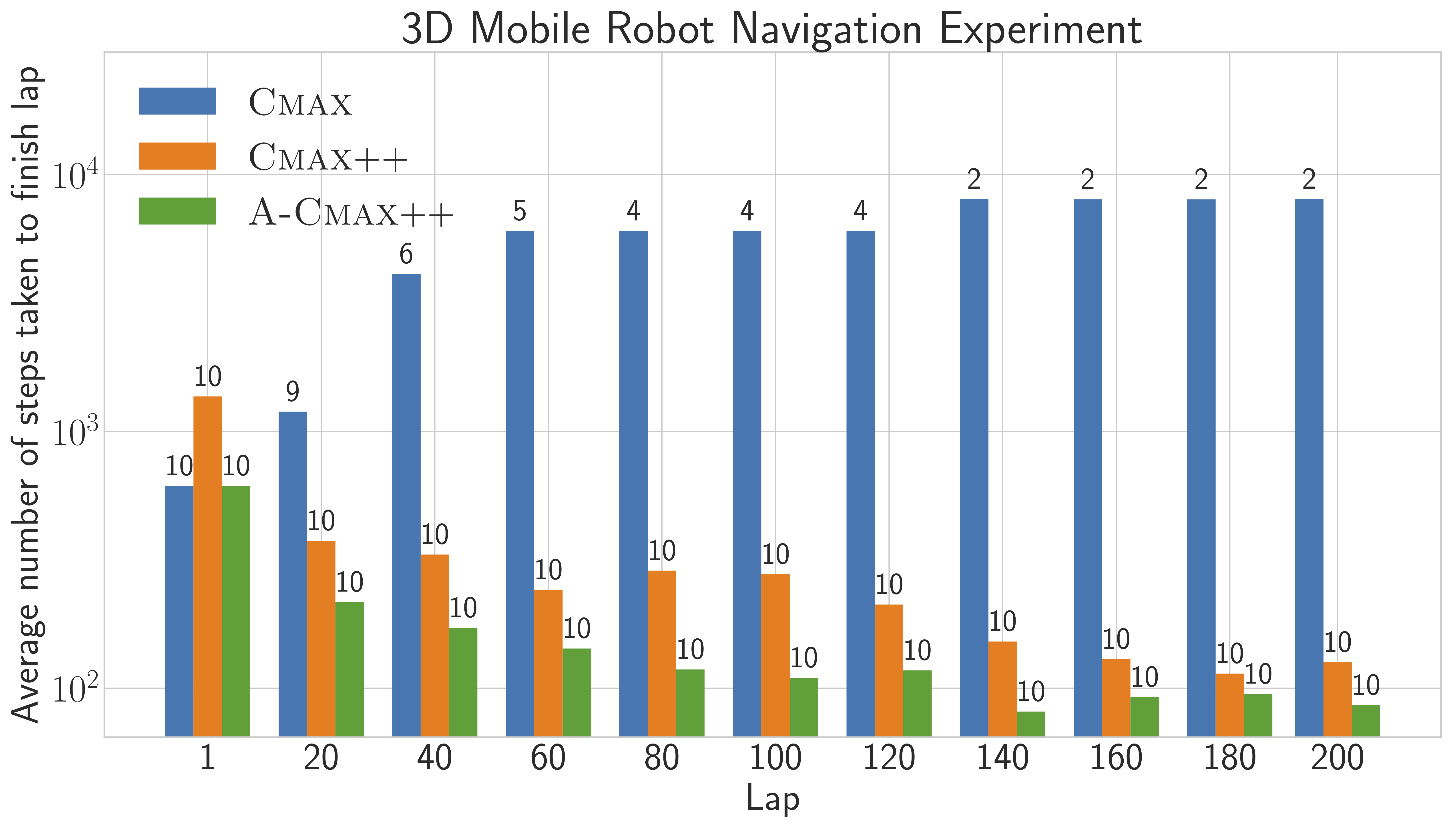
Fig. 4: Number of steps taken to finish a lap averaged across 10 instances each with 5 icy patches placed randomly around the track. The number above each bar reports the number of instances in which the robot was successful in finishing the respective lap within 10000 time steps.
As we expect, CMAX performs well in early laps computing paths with lower costs than CMAX++. However, after a few laps the robot using CMAX gets stuck within an icy patch and does not make any progress since all transitions taking it out of the icy patch have their costs inflated in previous laps. Thus, CMAX manages to finish $200$ laps in only $2$ out of $10$ instances. CMAX++, on the other hand, is suboptimal in initial laps, but converges to lower costs in later laps and finishes $200$ laps in all instances. Adaptive-CMAX++ also manages to finish $200$ laps in all instances but it outperforms both CMAX and CMAX++ in terms of cost of computed path in all laps by intelligently switching between them achieving goal-driven behavior in early laps and optimal behavior in later laps.
The second experiment uses the same setting as our motivating example where PR2 is trying to pick and place a heavy object from a start pose to a goal pose that is on a taller table. As the object is heavy, the arm cannot generate the required force in certain configurations and can only lift the object to small heights. The problem is represented as planning in large 7D discrete state space (the arm is 7-DOF) and the action space is a discrete set of $14$ actions corresponding to moving each dimension by a fixed offset in the postive and negative directions. The approximate model used for planning models the object as light and hence cannot capture the dynamics of the arm accurately when its lifting the object higher. The objective of the task is to pick and place the object for $20$ repetitions.
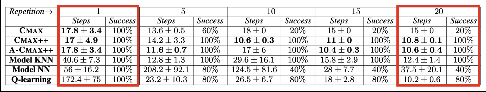
Fig. 5: Number of steps taken to reach the goal in 7D pick-and-place experiment for 5 instances, each with random start and obstacle locations. We report mean and standard error only among successful instances in which the robot reached the goal within 500 timesteps. The success subcolumn indicates percentage of successful instances.
We compare the performance of CMAX++ and Adaptive-CMAX++ against CMAX, residual model learning baselines and a model-free Q-learning baseline. For our model-based baselines, we have two variants - one which uses a global function approximation (neural network - NN) to learn the residual dynamics similar to previous works, and the other which uses a local function approximation (nearest neighbor regressors - KNN) to learn the residual dynamics. The model-free baseline is DQN which learns a residual component for the value function on top of an initial hardcoded value function that is obtained through extensive planning on the approximate model. Thus, all approaches start with the same initial value estimates.
Model-free Q-learning takes a large number of executions in the initial repetitions to estimate accurate Q-value estimates but in later repetitions computes paths with lower costs managing to finish all repetitions in 4 out of 5 instances. Among the residual model learning baselines, the KNN approximator is successful in all instances but takes a large number of executions to learn the true dynamics, while the NN approximator finishes all repetitions in only 2 instances. CMAX performs well in the initial repetitions but quickly gets stuck due to inflated costs and manages to complete the task for 20 repetitions in only 1 instance. CMAX++ is successful in finishing the task in all instances and repetitions, while improving performance across repetitions. Finally as expected, Adaptive-CMAX++ also finishes all repetitions, sometimes even having better performance than CMAX and CMAX++.
Discussion
Unlike CMAX, which was heavily goal-driven and tries to quickly find an alternative path, CMAX++ tries to identify if there are any incorrect transitions that lead to the goal with lower costs and exploits them in future replanning. Thus, CMAX++ leverages past experience and enables the planner to compute solutions containing such transitions. This makes CMAX++ especially useful in domains where learning the true dynamics online is a hopeless endeavor since it is too complex, such as deformable manipulation. CMAX++ also shines in domains where the dynamics vary over time due to reasons such as wear and tear, as it never tries to learn true dynamics and instead simply maintains model-free Q-value estimates.
CMAX is also suitable for these domains but has undesirable properties when applied to repetitive tasks and requires strong assumptions on the initial approximate model. CMAX++, on the other hand, needs the weak optimistic model assumption that is easier to satisfy and can improve task performance across repetitions in repetitive tasks. Note that even in the extreme case where the model is inaccurate everywhere in the state space, CMAX++ still works (essentially degrades to model-free Q-learning) while CMAX simply fails.
One could argue that the optimistic model assumption is still a very strong assumption in some domains where designing an initial optimistic model is difficult and requires extensive domain knowledge. While this is true, it is currently infeasible to relax this assumption further without resorting to global undirected exploration methods, which are terribly sample-inefficient, to ensure completeness. Maybe this is where practitioners need to draw the line on how much time one should spend on acquiring domain knowledge and designing good models, and what should be learned online during execution.
I hope this line of work convinces researchers that there is great value in extracting as much as possible out of the simplified and potentially inaccurate models that we have access to, before resorting to learning dynamics. The easy-to-implement nature of both CMAX and CMAX++ should enable widespread adoption as good baselines to compare against and as practical approaches that can be readily deployed.