I recently came across this book from Bertsekas that looked very interesting. It promises to provide a novel (geometric) interpretation of the methods that underlie the success of AlphaZero, AlphaGo, and TD-Gammon. I thought it would be interesting to take this as an opportunity to read the book, and have a blog post series on the key takeaways.
I think this will be a 3-part blog series with the following contents:
- Part 1 (this post): Notation, Bellman Operators, and geometric interpretation of value iteration.
- Part 2: Approximation in Value Space, one-step and multi-step lookahead, and certainty equivalent approximations.
- Part 3: Geometric interpretation of policy iteration, truncated rollout, and final remarks.
With that, let’s kick-off part 1.
Overview
Before I dive into the book, let me lay out an overview of the methodology underlying AlphaZero and TD-Gammon. They were both trained off-line extensively using neural networks and an approximate version of policy iteration. However, note that the AlphaZero player that was obtained off-line is not directly used during on-line play. Instead, a separate on-line player is used to select moves, based on multi-step lookahead minimization and a terminal position evaluator that was trained using experience with the off-line player. In a similar fashion, TD-Gammon (on-line) uses an off-line neural network-trained terminal position evaluator, and extends its on-line lookahead by rollout using the one-step lookahead player based on the position evaluator.
Bertsekas observes that
- The on-line player of AlphaZero plays much better than its extensively trained off-line player. This is due to the beneficial effect of exact policy improvement with long lookahead minimization, which corrects for the inevitable imperfections of the neural network-trained off-line player.
- The TD-Gammon player that uses long rollout plays much better than TD-Gammon without rollout. This is due to the beneficial effect of the rollout, which serves as a substitute for long lookahead minimization
This book answers why on-line player works so much better than directly using the off-line player.
The answer can be summarized as:
- Approximation in value space with one-step lookahead minimization amounts to a step of Newton’s method for solving Bellman’s equation
- The starting point for the Newton step is based on the results of off-line training, and may be enhanced by longer lookahead minimization and on-line rollout
Bertsekas also says the following which I believe is the major claim made in this book:
The major determinant of the quality of the on-line policy is the Newton step that is performed on-line, while off-line training plays a secondary role by comparison
With the motivation and the main contributions out of the way, its time for some notation to understand the insights behind the contributions.
Notation
The following notation will be used in all of the blog posts concerning this book. This is the same notation that Bertsekas uses in the book. Oddly, it differs from the usual RL notation that we are used to, so I will try to draw parallels in this section.
The dynamics are of the form, $$ x_{k+1} = f(x_k, u_k, w_k) $$
- States are denoted using $x_k \in X$ (same as $s$ in RL)
- Controls are denoted using $u_k \in U$ (same as $a$ in RL)
- The system has a random disturbance denoted by $w_k \in W$, which is governed by a probability distribution $P(\cdot|x_k, u_k)$ (we do not have a parallel for this as we assume the dynamics as a probability transition matrix, and $w$ serves the same purpose here)
- Stationary policies are denoted using $\mu \in M$ which map states to controls (same as $\pi$ in RL)
- Cost is denoted using $g(x_k, u_k, w_k)$ (same as $c(s, a)$ in RL, but note that the cost can depend on the noise as well here)
- Discount factor is denoted using $\alpha \in (0, 1]$ (same as $\gamma$ in RL)
We are primarily interested in minimizing the expected total cost $$ J_\mu(x_0) = \lim_{N \rightarrow \infty} \mathbb{E}[\sum_{k=0}^{N-1} \alpha^k g(x_k, \mu(x_k), w_k)] $$
- We use $J_\mu$ to denote the cost function of the policy $\mu$.
- The optimal cost function is denoted using $J^*$ which satisfies $J^*(x) = \inf_{\mu}J_\mu(x)$ for all states $x$.
Bellman Operators
To avoid unwieldy notation and to also encourage thinking of Bellman’s equations as operators, we define the following Bellman operators. Understanding this notation and properties of these operators is crucial for understanding the main takeaways presented in these blog posts.
- We use $TJ$ to denote the function that appears in the right-hand side of the Bellman’s equation, where for all $x$ we have $$ (TJ)(x) = \min_{u \in U(x)}\mathbb{E}[g(x, u, w) + \alpha J(f(x, u, w))] $$
- Also for each policy $\mu$, we introduce $T_\mu J$, which is defined at all $x$ as $$ (T_{\mu}J)(x) = \mathbb{E}[g(x, \mu(x), w)+ \alpha J(f(x, \mu(x), w))] $$
These two operators have the following properties:
- (Monotonic): $T, T_\mu$ are monotonic, i.e. if $J(x) \geq J’(x)$ for all $x$, then we have
- $(TJ)(x) \geq (TJ’)(x)$, and
- $(T_\mu J)(x) \geq (T_\mu J’)(x)$
- (Linear Operator): $T_\mu$ is a linear (actually, affine) operator in $J$
- (Concavity): $T$ is a concave function of $J$ since $(TJ)(x) = \min_{\mu \in M} (T_\mu J)(x)$ and pointwise minimum of linear functions is concave
The linearity of $T_\mu$ and the concavity of $T$ are the two main properties that enable the interpretation of policy improvement in AlphaZero-like approaches as Newton steps. They will also be crucial in our geometric interpretations of popular RL methods.
Geometric Interpretation of Value Iteration
Before we end part 1, I thought it would be nice for the readers to see how the above properties lend us a new (geometric) way of interpreting popular RL methods like value iteration. First, let’s use the operator notation to describe the value iteration algorithm.
We describe two versions of value iteration: the policy evaluation version, and the policy improvement version.
- (Policy Evaluation VI): $J_{k+1} = T_\mu J_k$ for iterations $k=0, 1, \cdots$
- (Policy Improvement VI): $J_{k+1} = TJ_k$ for iterations $k=0, 1, \cdots$
Both of the above value iteration approaches have a staircase-like construction in their geometric interpretation as shown below. First, we will show the geometric interpretation of policy evaluation VI.
Policy Evaluation Value Iteration
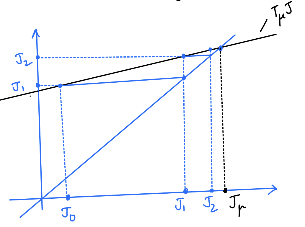
The above graph is the first of many in this blog post series. For all of these graphs, both X- and Y-axis denote the space of all cost functions $J$. The (blue) line going through the origin is always the $y=x$ line.
The above graph shows two iterations of the policy evaluation VI starting from $J_0$ and ending at $J_2$. The black line depicts the function that applies the operator $T_\mu$. Note that it is linear as we know $T_\mu$ is a linear operator. The point at which it intersects the $y=x$ line is represented by $J_\mu$, i.e. the cost of the policy $\mu$.
Starting from $J_0$, the first iteration applies the operator $T_\mu$ to get the next iterate $J_1$, which subsequently undergoes the same operation $T_\mu$ once more to get to $J_2$. Note that this repeated operation converges to $J_\mu$ as it is the fixed point of the operation $J = T_\mu J$.
Now, let’s see the geometric interpretation of policy improvement VI.
Policy Improvement Value Iteration
Couple of things to note here:
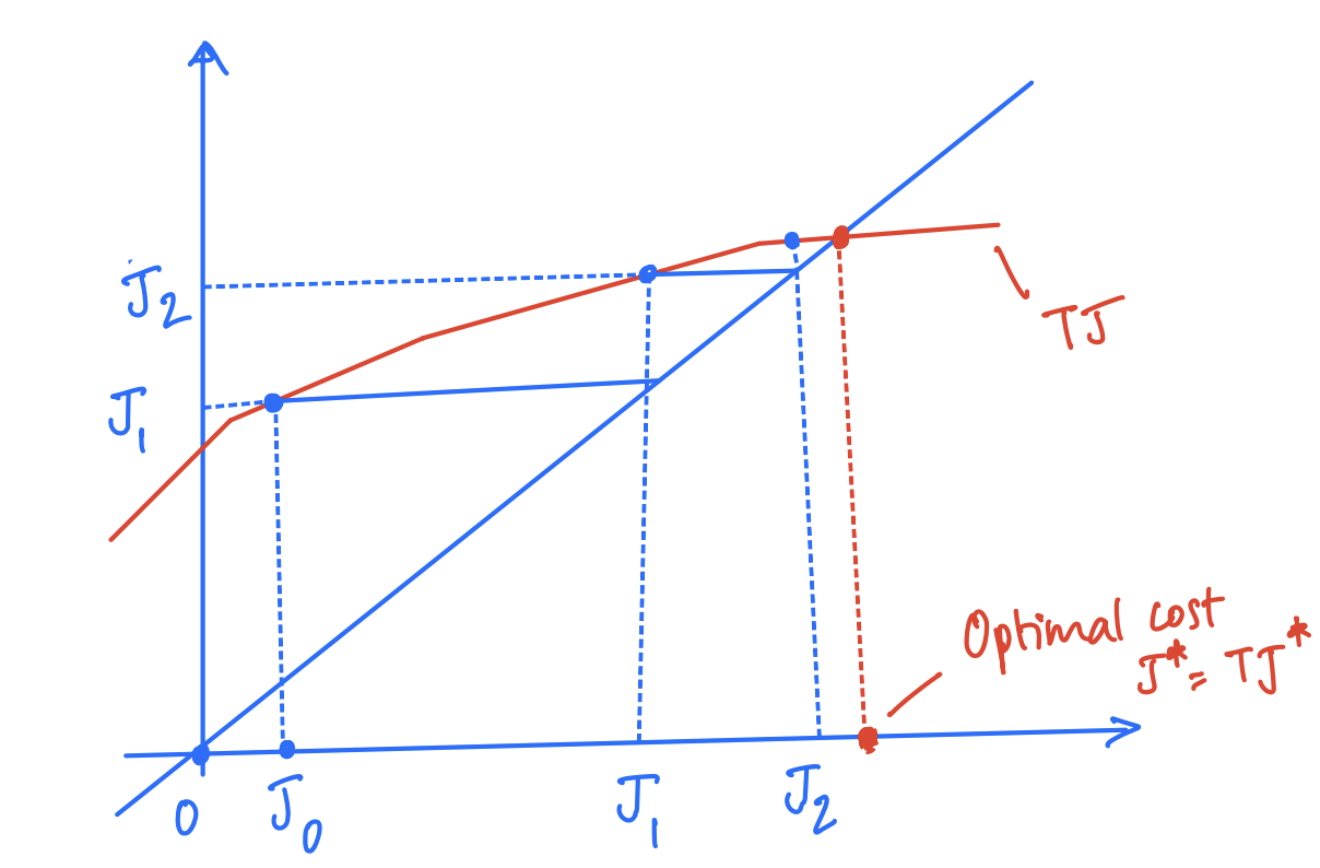
- The red line denotes the operator $T$, which we know is concave. Note that the function depicted in the above graph is not linear, but is concave.
- The point at which the red line intersects the $y=x$ line is represented by the optimal cost $J^*$ as it is the solution to $J = TJ$.
The above graph shows two iterations of the policy improvement VI. Starting from $J_0$, the first iteration applies the operator $T$ to get the next iterate $J_1$, which is used in the next iteration to apply $T$ once again to get $J_2$. This repeated operation would now converge to the optimal cost $J^*$ as it is the fixed point of the operation $J = TJ$.
Remarks
- The above two graphs show a neat geometric interpretation of the VI algorithms that I found very interesting. Bertsekas builds on these interpretations to understand more complex approaches such as multi-step lookahead minimization and truncated rollout.
- The two graphs belie the main difference between the two VI approaches (besides the linearity of $T_\mu$ and concavity of $T$): computing $T_\mu J$ can be much less computationally demanding than computing $TJ$ as it does not involve minimization over the control dimension.
- Note that the line representing $T_\mu$ can have one of three cases:
- The line has slope less than $45$ degrees, so it intersects the $y=x$ line at a unique point corresponding to $J_\mu$ which is a solution of $J = T_\mu J$
- The line has slope greater than $45$ degrees, so it intersects the $y=x$ line at a unique point corresponding to solution of $J = T_\mu J$ but not equal to $J_\mu$. $J_\mu$ is not real-valued and $\mu$ is an unstable policy
- The line has slope exactly $45$ degrees, in which case it either has infinite or no solution at all.
Epilogue
This is a good point to end this part of the series. The next two posts get to the meat of the insights from the book, and build upon these geometric interpretations. Stay tuned!