This is part 2 of the blog post series on this book from Bertsekas, and its key takeaways.
Let’s pick it up from where we left off in part 1. Will highly recommend readers to check out part 1 before continuing in part 2, as some important notation and ideas were described there, which will be relevant in this part.
As a recap, here’s the breakdown for the 3-part blog series:
- Part 1: Notation, Bellman Operators, and geometric interpretation of value iteration.
- Part 2 (this post): Approximation in Value Space, one-step and multi-step lookahead, and certainty equivalent approximations.
- Part 3: Geometric interpretation of policy iteration, truncated rollout, and final remarks.
With that, let’s kick-off part 2.
Approximation in Value Space
Bertsekas calls the on-line player approach of AlphaZero, approximation in value space, as this involves a lookahead minimization combined with truncated rollout and a terminal position evaluator (a.k.a value estimator.) For the purposes of this post, let’s ignore the truncated rollout part, and focus on effects of lookahead minimization and value estimator. We will examine the effect of truncated rollout in part 3.
For readers who are unfamiliar with the AlphaZero online player approach, the following figure from the book is an apt summary:
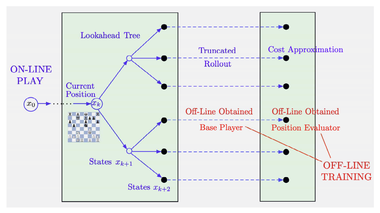
The approach of using an approximate cost estimator for the leaf states to compute a policy at state $x_0$ is referred to as approximation in value space. This approach is motivated by re-examining Bellman’s equation from part 1:
$$ \mu^*(x) \in \arg\min_{u \in U(x)}\mathbb{E}[g(x, u, w) + \alpha J^*(f(x, u, w))] $$
where $J^*$ is the optimal cost-to-go function. However, the off-line trained cost estimator $\tilde{J}$ is an approximation of $J^*$. Substituting $\tilde{J}$ in place of $J^*$ in the Bellman’s equation results in the one-step lookahead approximation in value space approach:
$$ \tilde{\mu}(x) \in \arg\min_{u \in U(x)}\mathbb{E}[g(x, u, w) + \alpha \tilde{J}(f(x, u, w))] $$
The above minimization yields a new stationary policy $\tilde{\mu}$ with cost-to-go $J_{\tilde{\mu}}$. Note that the cost of $\tilde{\mu}$ is not $\tilde{J}$. Instead it is $J_{\tilde{\mu}}$ which satisfies $T_{\tilde{\mu}}J_{\tilde{\mu}} = J_{\tilde{\mu}}$.
The key observation from Bertsekas is that:
The change from $\tilde{J}$ to $J_{\tilde{\mu}}$ will be interpreted as a step of Newton’s method for solving Bellman’s equation
This will suggest that $J_{\tilde{\mu}}$ is closer to $J^*$ and obeys a superlinear convergence relation, i.e.
$$ \lim_{\tilde{J} \rightarrow J^*} \frac{J_{\tilde{\mu}}(x) - J^*(x)}{\tilde{J}(x) - J^*(x)} = 0 $$
Furthermore, he also makes another crucial observation:
For $\ell$-step lookahead minimization, it can be interpreted as Newton’s method for solving Bellman’s equation, starting from $\hat{J}$, which is an “improvement” over $\tilde{J}$. In particular, $\hat{J}$ is obtained from $\tilde{J}$ by applying $(\ell-1)$ successive value iterations.
We will spend the rest of this post understanding how the above two observations can be drawn from a geometric perspective, thereby understanding the core premise of the book which is to answer why the on-line player works so much better than directly using the off-line player?
Geometric Interpretation of One-step Lookahead Policy
The one-step lookahead policy is computed as follows for any state $x$:
$$ \min_{u \in U(x)} \mathbb{E}[\underbrace{g(x, u, w)}_{\text{First step}} + \underbrace{\alpha \tilde{J}(f(x, u, w))}_{\text{Future}}] $$
The above minimization yields a control $\tilde{u}$ at state $x$, which defines the one-step lookahead policy $\tilde{\mu}$ via $\tilde{\mu}(x) = \tilde{u}$. In other words, $\tilde{\mu}$ is defined using
$$ \tilde{\mu}(x) \in \arg\min_{u \in U(x)} \mathbb{E}[g(x, u, w) + \alpha \tilde{J}(f(x, u, w))] $$
which is the same as saying, $T_{\tilde{\mu}}\tilde{J} = T\tilde{J}$. Geometrically, the graph of $T_{\tilde{\mu}}J$ just touches the graph of $TJ$ at $\tilde{J}$. This can be interpreted geometrically using the following figure.
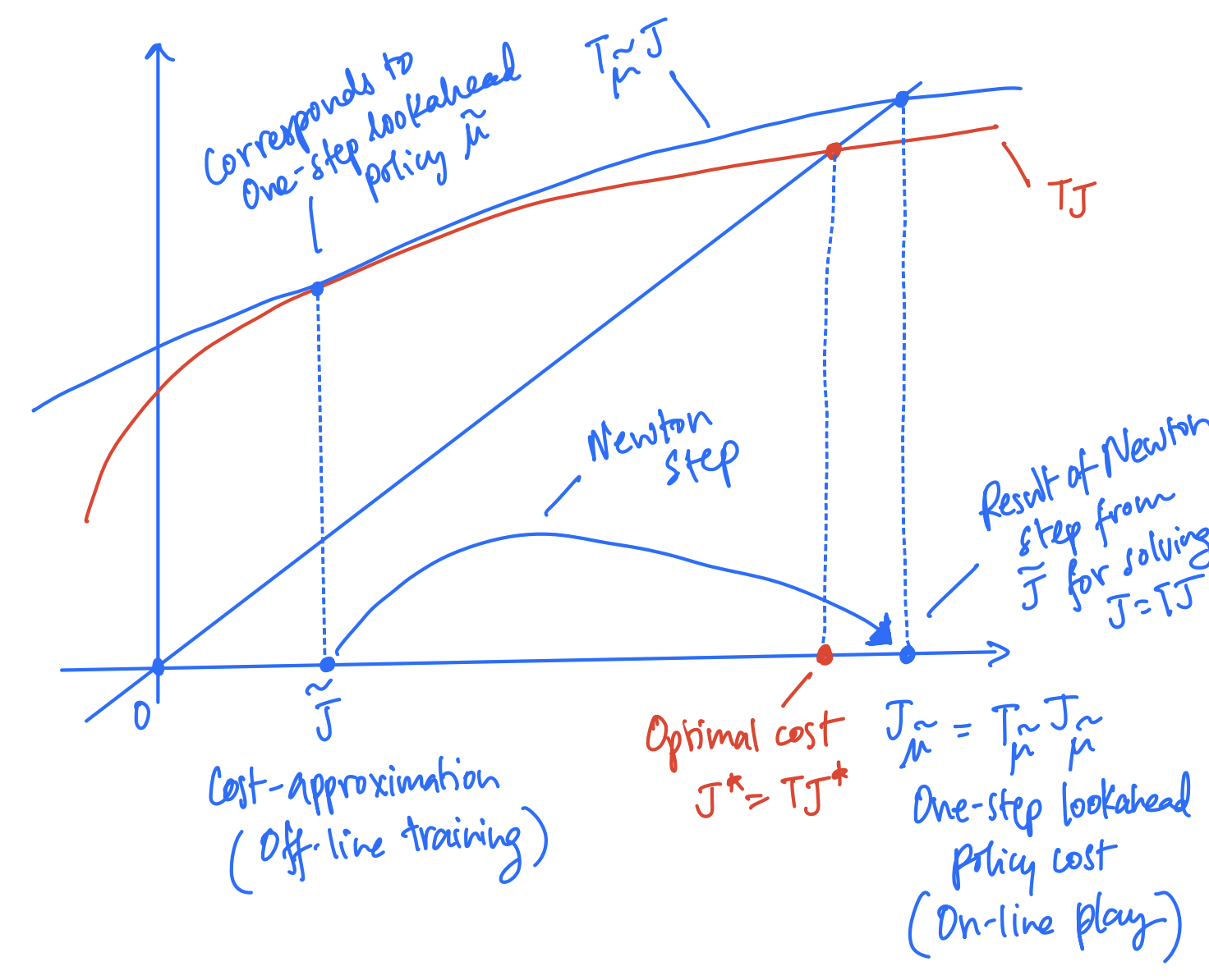
The above figure can be understood through the following:
- From part 1, we know that $T_{\tilde{\mu}}$ is a linear function (in $J$) and hence is represented using the blue line in the above graph,
- $T$ is a concave function and is represented using the red curve,
- The line corresponding to $T_{\tilde{\mu}}$ intersects the concave curve of $T$ at the starting point $\tilde{J}$,
- The blue line $T_{\tilde{\mu}}$ intersects the $y=x$ line at the point $J_{\tilde{\mu}}$ as it is the solution to the fixed point equation $T_{\tilde{\mu}}J = J$, and
- The red curve $T$ intersects the $y=x$ line at the point $J^*$ (the optimal cost) as it is the solution to the fixed point equation $TJ = J$.
The update from starting point $\tilde{J}$ to $J_{\tilde{\mu}}$ can be seen as a result of applying one step of Newton’s method for finding the fixed point of the equation $TJ = J$ at the start point $\tilde{J}$. This can be inferred from the following observations:
- $T_{\tilde{\mu}}$ is the linearization of $T$ at $\tilde{J}$
- $J_{\tilde{\mu}}$ corresponds to the point of intersection of the linearization $T_{\tilde{\mu}}$ with the line $y=x$, i.e. it is the solution for $T_{\tilde{\mu}}J = J$
Thus, this is exactly like performing one step of Newton’s method. Note that the new iterate $J_{\tilde{\mu}}$ is significantly closer to optimal cost $J^*$ than the start point $\tilde{J}$. Repeating this process over several iterations will quickly get us close to the optimal cost $J^*$.
We can also make a similar geometric interpretation for the $\ell$-step lookahead policy.
Geometric Interpretation of $\ell$-step lookahead policy
The $\ell$-step lookahead policy is computed as follows for any state $x$:
$$ \min_{u_k, \mu_{k+1}, \cdots, \mu_{k+\ell-1}} \mathbb{E}[\underbrace{g(x_k, u_k, w_k) + \sum_{i=k+1}^{k+\ell-1} \alpha^{i-k}g(x_i, \mu_i(x_i), w_i)}_{\text{First } \ell \text{ steps}} + \underbrace{\alpha^\ell \tilde{J}(x_{k+\ell})}_{\text{Future}}] $$
The above minimization yields a control $\tilde{u}_k$ and a sequence of policies $\tilde{\mu}_{k+1}, \cdots, \tilde{\mu}_{k+\ell-1}$. The control $\tilde{u}_k$ is applied at state $x_k$, and defines the $\ell$-step lookahead policy $\tilde{\mu}$ via $\tilde{\mu}(x_k) = \tilde{u}_k$. The sequence of policies $\tilde{\mu}_{k+1}, \cdots, \tilde{\mu}_{k+\ell-1}$ is discarded.
In other words, $\tilde{\mu}$ is defined using
$$ \tilde{\mu}(x_k) \in \arg\min_{u_k \in U(x)} \min_{\mu_{k+1}, \cdots, \mu_{k+\ell-1}} \mathbb{E}[g(x_k, u_k, w_k) + \sum_{i=k+1}^{k+\ell-1} \alpha^{i-k}g(x_i, \mu_i(x_i), w_i) + \alpha^\ell \tilde{J}(x_{k+\ell})] $$
which is the same as $T_{\tilde{\mu}}\tilde{J} = T^\ell\tilde{J} = T(T^{\ell-1}\tilde{J})$. We can reformulate this as $T_{\tilde{\mu}}\tilde{J} = T\hat{J}$ where $\hat{J} = T^{\ell-1}\tilde{J}$.
Few remarks can be made from the above bellman operator interpretation:
- Note that the $\ell$-step lookahead minimization involves $\ell$ successive value iterations, but only the first of these iterations has a Newton step interpretation
- The first step of lookahead is the Newton step (from $T^{\ell-1}\tilde{J}$ to $J_{\tilde{\mu}}$) and the rest of the steps are simply preparation for the Newton step (i.e. $\tilde{J}$ to $T^{\ell-1}\tilde{J}$.)
The $\ell$-step lookahead minimization can be interpreted geometrically using the following figure.
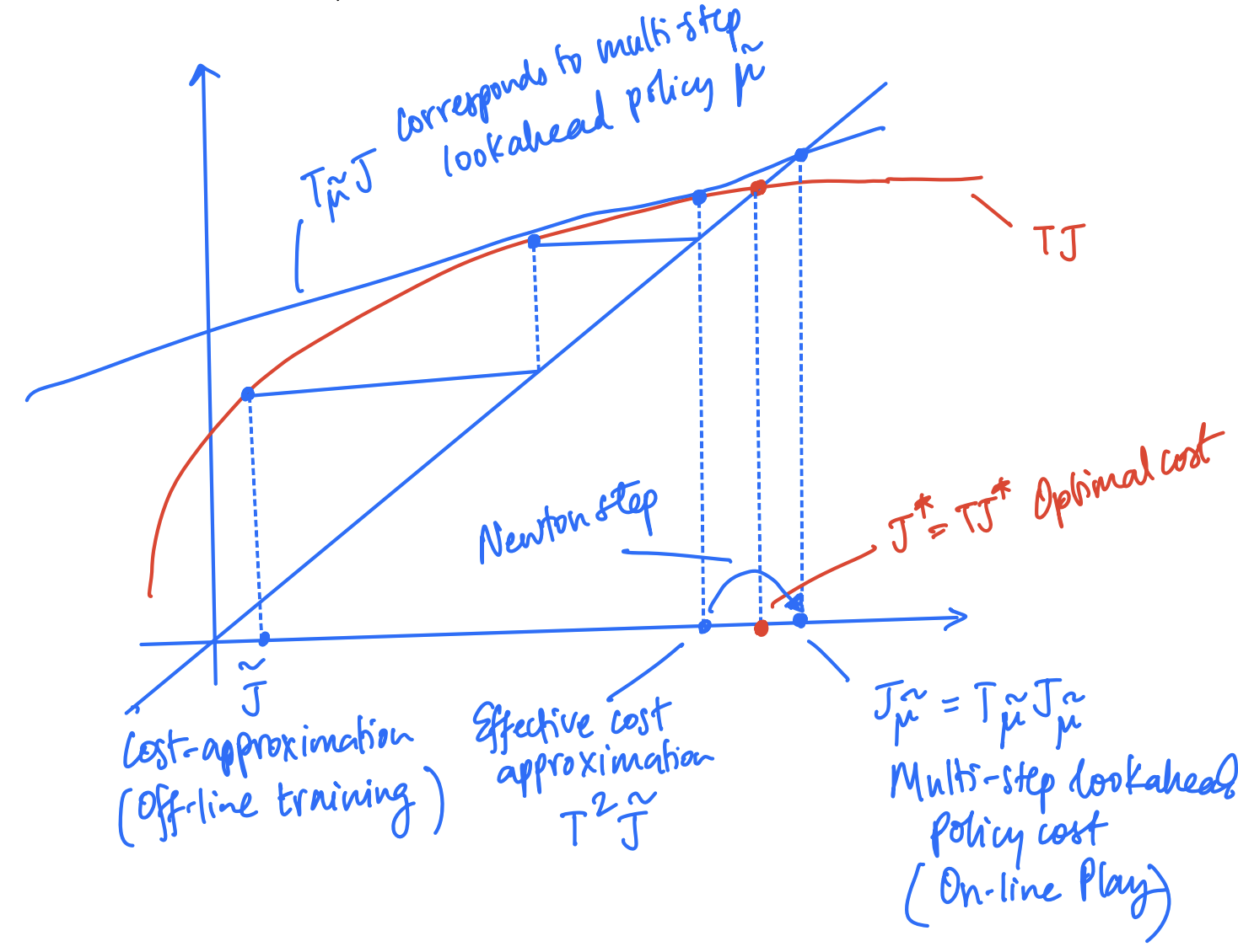
The above figure can be understood through the following:
- The blue line corresponding to $T_{\tilde{\mu}}$ intersects the red curve of $T$ at $\hat{J} = T^{\ell-1}\tilde{J}$ ($= T^2\tilde{J}$ in this example) as it is the fixed point of the equation $T_{\tilde{\mu}}J = TJ$
- To get to $\hat{J} = T^{\ell-1}\tilde{J}$ from the start point $\tilde{J}$, we need to perform $(\ell-1)$ successive value iterations (as shown by the staircase construction above.)
- To perform the first step (from $\hat{J}$ to $J_{\tilde{\mu}}$,) we linearize $T$ at $\hat{J} = T^{\ell-1}\tilde{J}$ and compute its intersection with the $y=x$ line to give $J_{\tilde{\mu}}$.
Thus, the update from $T^{\ell-1}\tilde{J}$ to $J_{\tilde{\mu}}$ corresponds to one-step of Newton’s method for finding the fixed point of the equation $TJ = J$ at the point $T^{\ell-1}\tilde{J}$, which itself is constructed by performing $(\ell - 1)$ successive value iterations from the start point $\tilde{J}$.
Remarks
- From the above two interpretations, Bertsekas claims that most of the benefit of the on-line player comes from the Newton’s step that is performed through lookahead minimization
- The off-line training only prepares the starting point of the Newton step, and is not as essential as the on-line Newton step
- The effect of off-line training can be minimized by increasing the lookahead depth, as the $(\ell-1)$ successive value iterations can bring the very coarse approximation $\tilde{J}$ (from off-line training) close to $J^*$, thereby alleviating the need for accurate approximations from off-line training
- As we will see in part 3, truncated rollout is also another way to reduce the impact of off-line training and enhance the starting point of Newton step
- Finally it is to be noted that approximation in value space computes $J_{\tilde{\mu}}$ differently than policy iteration (as we will see in part 3.) It does not explicitly compute $J_{\tilde{\mu}}$; instead, the control is applied to the system and cost is accumulated accordingly. Thus, values of $J_{\tilde{\mu}}$ are implicitly computed only for those states $x$ that are encountered in the system trajectory generated on-line.
Certainty Equivalent Approximations
The above interpretations can beg a new question: Can we construct new approaches by using other approximations to $J^*$ in Bellman’s equation?. The answer is YES, and we will show an example in this section.
We can replace the Bellman operators $T$ and $T_\mu$ with deterministic variants:
$$ (\bar{T}J)(x) = \min_{u \in U(x)} g(x, u, \bar{w}) + \alpha J(f(x, u, \bar{w})) $$ $$ (\bar{T}_\mu J)(x) = g(x, \mu(x), \bar{w}) + \alpha J(f(x, \mu(x), \bar{w})) $$ where $\bar{w}$ is a deterministic variable, and unlike $w$ which was stochastic noise.
Using the deterministic operators greatly simplifies $\ell$-step lookahead as there are no stochastic steps. However, it is to be noted that using deterministic steps for all $\ell$ steps leads to a Newton step for fixed points of $\bar{T}$, not $T$, which is not what we want.
This can be circumvented by using stochastic step for the first step, and deterministic steps for the remaining $(\ell-1)$ steps, i.e.
$$ T_{\bar{\mu}}(\bar{T}^{\ell-1} \tilde{J}) = T(\bar{T}^{\ell-1}\tilde{J}) $$ This performs a Newton step to find fixed point of $T$ starting from $\bar{T}^{\ell - 1}\tilde{J}$. The performance penalty is minimal if $\bar{T}^{\ell-1}\tilde{J}$ is “close” to $J^*$.
We can similarly construct a more general approximation scheme where, we use any approximation $\hat{J}$ that is sufficiently “close” to $J^*$ and obtain a policy $\tilde{\mu}$ using
$$ T_{\tilde{\mu}}\hat{J} = T\hat{J} $$
which involves a Newton step from $\hat{J}$ to $J_{\tilde{\mu}}$.
Epilogue
This part presented one of the major takeaways from Bertsekas book, namely understanding why lookahead minimization is performed in on-line play rather than directly using off-line trained policy. Furthermore, we also understand how much of an impact off-line training can have in approximation in value space approaches, and how to mitigate its effects using lookahead.
In the next (and final) part, we will explore the other methodology used by AlphaZero, truncated rollout, to mitigate the effect of off-line training and also interpret policy iteration (another fundamental RL algorithm) geometrically. By the end of the next part, we will understand all the key takeaways from the book and also be equipped with an arsenal of geometric interpretations that we can use to analyze future RL algorithms.