We will continue with part 3 (and the final part) of the blog post series on this book by Bertsekas. As always, I would highly recommend the readers to start with part 1 and part 2 before continuing in part 3, as all of the notation used in this post is introduced in the previous parts.
As a recap, here’s the breakdown for the 3-part blog series:
- Part 1: Notation, Bellman Operators, and geometric interpretation of value iteration.
- Part 2: Approximation in Value Space, one-step and multi-step lookahead, and certainty equivalent approximations.
- Part 3 (this post): Geometric interpretation of policy iteration, truncated rollout, and final remarks.
Let’s begin!
Policy Iteration
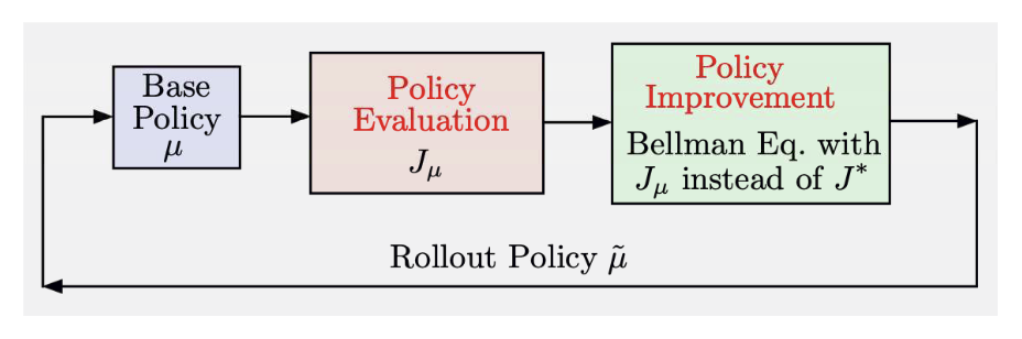
Another major class of RL approaches are based on Policy Iteration (PI), which involves repeated application of two steps:
- Policy Evaluation:
- Given a policy $\mu$, evaluate its cost $J_\mu$
- This can be done by solving the Bellman equation for $\mu$: $J = T_\mu J$, or by Monte-carlo methods that involve rolling out the policy $\mu$ and averaging cost incurred, or by other sophisticated methods such as Temporal Difference (TD) methods
- Policy Improvement:
- Given cost $J_\mu$, perform one-step lookahead minimization (explained in part 2) to obtain a new policy $\tilde{\mu}$
The above procedure is summarized in the following figure from the book:
Thus, PI generates a sequence of policies ${\mu^{k}}$ through:
- Policy Evaluation: $J_{\mu^k} = T_{\mu^k} J_{\mu^k}$
- Policy Improvement:$T_{\mu^{k+1}} J_{\mu^k} = TJ_{\mu^k}$
Note that the policy improvement update is the one-step lookahead minimization that we explored in part 2. Thus, policy improvement can be interpreted as the Newton step starting from $J_{\mu^k}$ that yields policy $\mu^{k+1}$ as the one-step lookahead policy.
Geometric Interpretation of Policy Iteration
Since policy improvement is the same as one-step lookahead minimization, and the policy evaluation operation can be done by solving the Bellman equation for base policy $\mu$, we can borrow the tools we built in part 1 and 2 to come up with the following geometric interpretation.
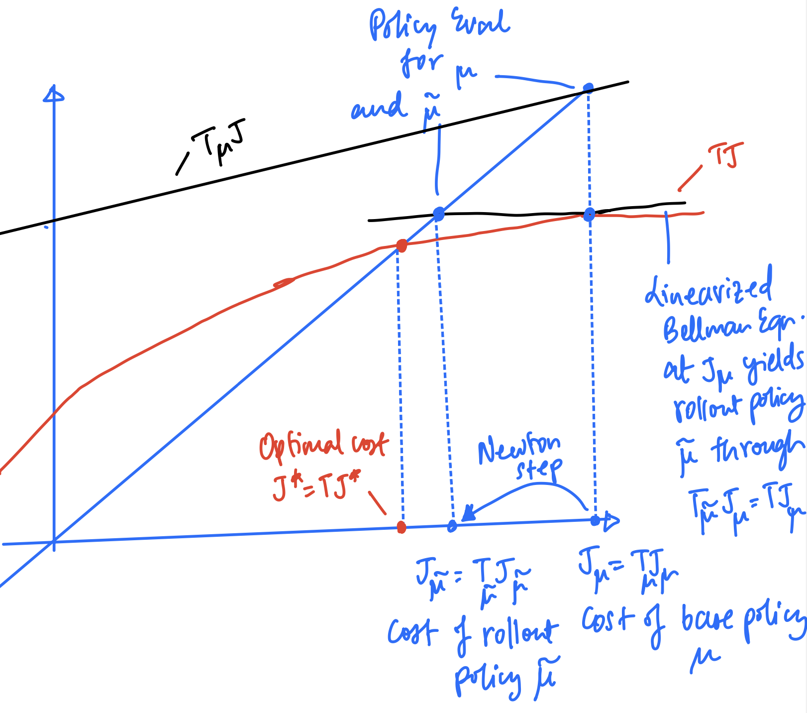
The above graph can be understood through the following:
- To evaluate the base policy $\mu$, we find the intersection of the line representing $T_\mu$ with the $y=x$ line, to give the cost $J_\mu$
- To perform policy improvement (a.k.a one-step lookahead minimization,) we linearize the curve representing $T$ at $x=J_\mu$ to get the line representing $T_{\tilde{\mu}}$ where $\tilde{\mu}$ is the one-step lookahead (or rollout) policy
- The line representing $T_{\tilde{\mu}}$ intersects the $y=x$ line at the cost of the lookahead policy giving us $J_{\tilde{\mu}}$
- Thus, the policy improvement operation is a Newton step from the cost of the base policy $J_\mu$ to the cost of the lookahead policy $J_{\tilde{\mu}}$
- Note that unlike VI and approximation in value space, the initial iterate of the Newton step $J_\mu$ always satisfies $J_\mu \geq J^*$ as it is the cost of a policy (and $J^*$ is the optimal cost)
Note that if the curve $T$ is nearly linear (i.e. has small curvature,) then the lookahead policy’s performance $J_{\tilde{\mu}}$ is close to optimal $J^*$, even if the base policy $\mu$ is far from optimal.
Furthermore, the Newton step interpretation gives us an error rate
$$ \lim_{J_\mu \rightarrow J^*} \frac{J_{\tilde{\mu}}(x) - J^*(x)}{J_\mu(x) - J^*(x)} \rightarrow 0 $$
that has superlinear convergence.
Truncated Rollout
Truncated rollout is the final piece of the puzzle that enables the use of any cost approximation $\tilde{J}$ along with a base policy $\mu$ to approximate the cost $J_\mu$, thus avoiding the possibly expensive step of policy evaluation.
Going back to the AlphaZero approach figure that we saw in part 2 (figure is from the book):
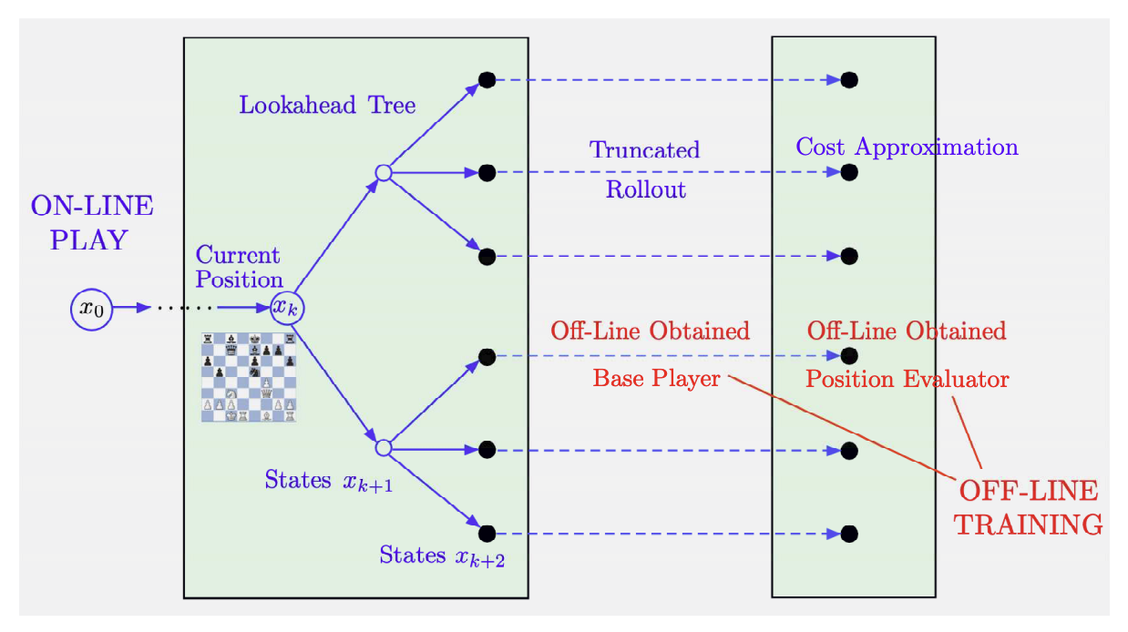
Note that the cost obtained by using the base policy $\mu$ for $m$ steps followed by terminal cost approximation $\tilde{J}$, is given by $T_{\mu}^m \tilde{J}$, i.e it is the result of applying $m$ iterations of policy evaluation VI corresponding to $\mu$ starting from $\tilde{J}$.
Thus, a one-step lookahead policy with $m$ steps of truncated rollout results in the policy $\tilde{\mu}$ that satisfies:
$$ T_{\tilde{\mu}} (T_\mu^m \tilde{J}) = T (T_\mu^m \tilde{J}) $$
This can also be extended to the general case of $\ell$-step lookahead (from part 2) as follows:
$$ T_{\tilde{\mu}} (T^{\ell-1} T_\mu^m \tilde{J}) = T (T^{\ell - 1} T_\mu^m \tilde{J}) $$
This can be interpreted geometrically using the following figure for ($m = 3$ and $\ell = 1$)
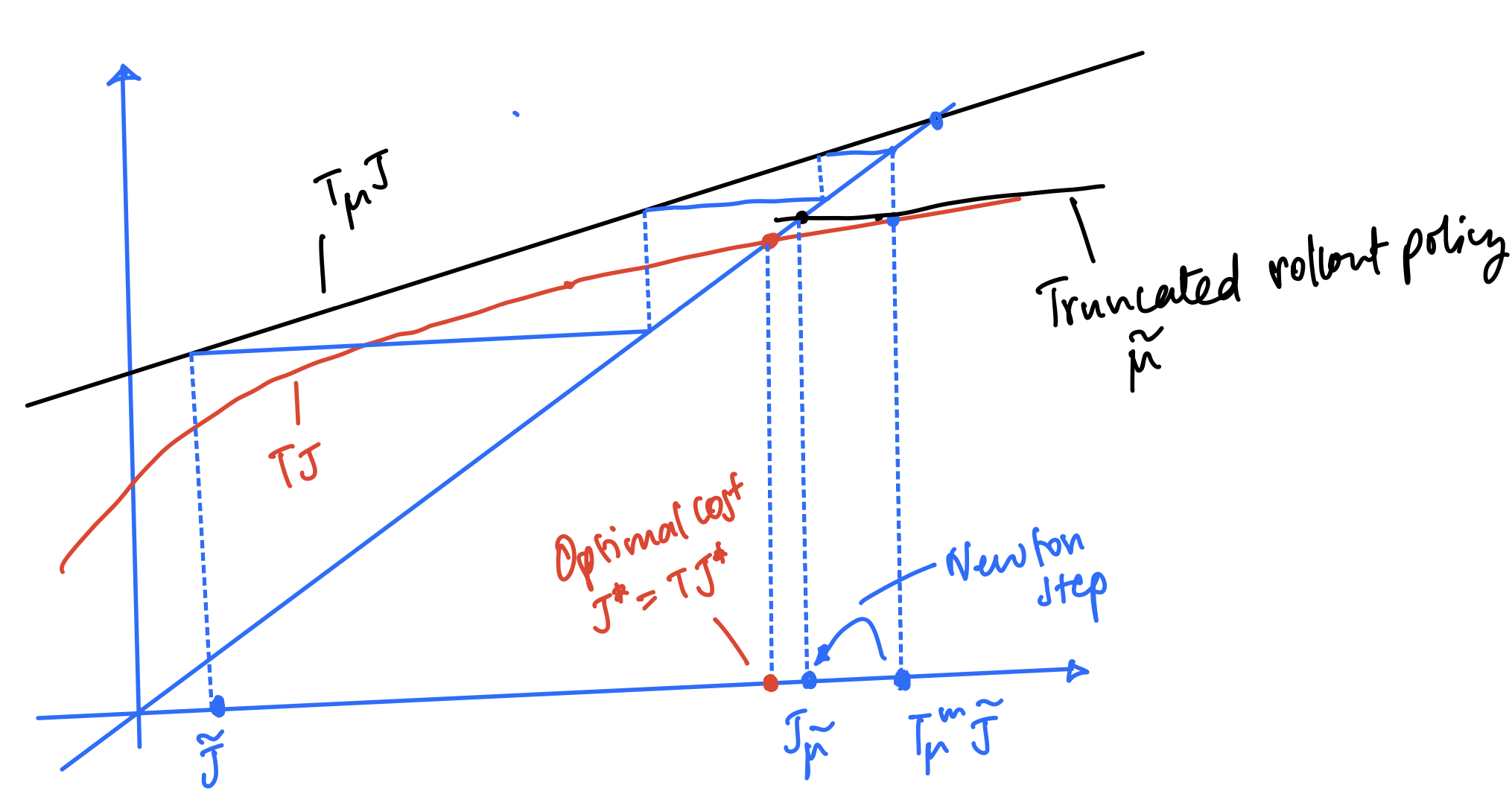
Observe that truncated lookahead with $ell$-step lookahead, followed by $m$-steps of base policy $\mu$ is an economical alternative to $(\ell+m)$-step lookahead.
Final Remarks
To conclude this blog post series, I wanted to list the main takeaways that I had from reading Bertsekas’ book:
- Larger values of $\ell$ for $\ell$-step lookahead is beneficial as it brings the starting point of the Newton step $T^{\ell-1}\tilde{J}$ closer to the optimal cost $J^*$
- However, it is only the first step of $\ell$-step lookahead that contributes to Newton step, while the remaining $(\ell-1)$ steps are far less-effective first order (or VI, in this case) iterations
- Larger values of $m$ for $m$-step truncated rollout brings the starting point of the Newton step $T_{\mu}^m\tilde{J}$ closer to $J_\mu$, and not $J^*$
- Thus, increasing $m$ beyond a certain point can be counter-productive
- Lookahead minimization is considerably more computationally expensive than truncated rollout. This, it is always preferable (computationally) to use larger values of $m$ than larger values of $\ell$.
Interesting Questions
Is lookahead by rollout an economic substitute for lookahead by minimization?
YES. For a given computational budget, judiciously balancing $m$ and $\ell$ tends to give a much better lookahead policy than simply increasing $\ell$ as much as possible, while setting $m=0$.
Why not just train a policy network and use it without online play?
The question is asking, in other words, whether using only approximation in policy space to learn a policy that can be used online is good enough. It does have the advantage of fast online inference (directly invoking the learned policy.) However, the offline trained policy may not perform nearly as well as the corresponding one-step or multi-step lookahead policy because it lacks the power of the associated exact Newton step
This concludes the blog post series. Please reach out in the comments or directly to me if you have any questions or corrections.